Random Forest: A Complete Beginner's Guide
Before We Start: The Core Idea in One Sentence
Random Forest builds a large number of deliberately different decision trees on random subsets of your data and random subsets of your features, then combines their predictions. A crowd of imperfect but diverse experts reliably outperforms any single expert.
1. Why Ensembles Work: Wisdom of Crowds
In 1906, statistician Francis Galton visited a county fair and observed an ox-weight-guessing competition. About 800 villagers each wrote down a guess. No single person was accurate, but the median of all guesses was 1,207 lb. The actual weight was 1,198 lb. The crowd was within 0.8%.
This phenomenon, that aggregating many independent imperfect estimates beats any individual estimate, is called the wisdom of crowds. Random Forest is its machine learning incarnation.
Formally, suppose you have \(B\) classifiers, each making an independent error with probability \(p < 0.5\). The probability that more than half of them are wrong (i.e., the majority vote is wrong) follows the binomial distribution:
For \(B = 100\) trees each with error rate \(p = 0.30\), the majority-vote error is approximately 0.0009%, compared to 30% for any single tree. That dramatic drop is the power of ensembles.
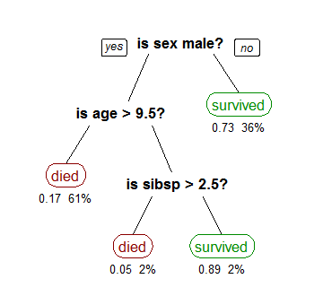
2. Prerequisites: Decision Trees in 5 Minutes
Random Forest is built on decision trees, so you need to understand them first. A decision tree recursively splits the training data at the feature value that best separates the classes.
2.1 Gini Impurity
The most common split criterion in Random Forest (and the default in scikit-learn) is Gini impurity, which measures how often a randomly chosen element would be incorrectly labelled if it were randomly labelled according to the class distribution at that node.
For a node containing \(n\) samples across \(K\) classes, where \(p_k\) is the fraction of samples belonging to class \(k\):
Interpretation of extremes:
- \(G = 0\): the node is pure. All samples belong to one class, so no more splitting is needed.
- \(G = 0.5\): for a binary problem, samples are split 50/50. This is maximum impurity. Knowing the node label tells you nothing.
Example: A node has 10 samples: 7 class A, 3 class B.
2.2 Entropy and Information Gain
Entropy (used in the ID3 / C4.5 algorithms) measures uncertainty using Shannon's information theory:
For the same node (7A, 3B):
Information Gain is the reduction in entropy achieved by a split:
where \(S\) is the current node, \(f\) is the feature being tested, and \(S_v\) is the subset where feature \(f\) takes value \(v\).
Gini vs Entropy: Both produce very similar trees in practice. Gini is slightly faster to compute (no logarithm) and is the scikit-learn default. Entropy can produce slightly more balanced trees.
2.3 How a Tree Grows
The CART (Classification and Regression Trees) algorithm builds a binary tree greedily:
- At the current node, consider every feature and every possible split threshold.
- Choose the split that minimises the weighted Gini impurity of the two child nodes:
\[ \text{Gini}_{\text{split}} = \frac{n_L}{n} G_L + \frac{n_R}{n} G_R \]
- Recursively repeat for each child node.
- Stop when a stopping condition is met: pure node, minimum samples, maximum depth, etc.
The critical weakness of a single tree: Grown to full depth, a decision tree memorises the training data perfectly (zero training error) but generalises poorly. It overfits. Random Forest solves this by averaging many trees, each trained on slightly different data.
3. Bagging: Bootstrap Aggregating
Bagging (short for Bootstrap Aggregating), proposed by Leo Breiman in 1996, is the foundation of Random Forest. The idea is:
- Bootstrap: From your training set of \(n\) samples, draw \(n\) samples with replacement to create a new dataset. Some original samples appear multiple times; others are omitted entirely. On average, ~36.8% of samples are left out and form the Out-of-Bag set (covered in Section 7).
- Train: Fit a full decision tree on the bootstrap sample.
- Repeat: Do steps 1–2 \(B\) times, producing \(B\) trees.
- Aggregate: For a new input, collect the prediction of each tree and return the majority vote (classification) or mean (regression).

Why does bootstrap sampling help?
Each bootstrap sample is a slightly different view of the data. Trees trained on different samples make different errors, and different errors cancel out when you average. This reduces variance without increasing bias, which is the key insight.
Mathematically, if each tree has variance \(\sigma^2\) and the trees are uncorrelated (\(\rho = 0\)), the variance of the average prediction is:
In practice, trees are correlated (they all train on the same features, so strong features appear in most trees), so the variance reduction is:
As \(B \to \infty\), this approaches \(\rho \sigma^2\). The remaining variance is entirely due to inter-tree correlation \(\rho\). This is exactly the problem that Random Forest's feature randomness solves.
4. Random Forest = Bagging + Feature Randomness
Random Forest, introduced by Leo Breiman in 2001, adds one crucial modification to bagging: at each split, only a random subset of \(m\) features is considered, rather than all \(p\) features.
| Algorithm | Bootstrap samples | Feature subsampling at each split |
|---|---|---|
| Single Decision Tree | No | All \(p\) features |
| Bagging | Yes | All \(p\) features |
| Random Forest | Yes | Random \(m \ll p\) features |
Recommended defaults for \(m\):
- Classification: \(m = \lfloor\sqrt{p}\rfloor\)
- Regression: \(m = \lfloor p/3 \rfloor\)
Why this extra step? Without feature subsampling, all trees in a bagged ensemble tend to use the same dominant features near the root. This makes the trees highly correlated (\(\rho\) stays high), limiting variance reduction. By forcing each tree to consider only a random subset of features at each split, we decorrelate the trees. Even if one feature is overwhelmingly predictive, many trees will not have access to it at key splits and will find alternative patterns. The ensemble correlation \(\rho\) drops, and the ensemble variance falls further.
5. The Complete Math
5.1 Bootstrap Sampling
Given a training set \(\mathcal{D} = \{(\mathbf{x}_1, y_1), \ldots, (\mathbf{x}_n, y_n)\}\), bootstrap sample \(b\) is drawn as:
The probability that any given sample is excluded from bootstrap \(b\):
So about 36.8% of training points form the Out-of-Bag (OOB) set for each tree.
5.2 Tree Construction (Formal)
For bootstrap sample \(b\), build tree \(\hat{f}^b\) using the CART algorithm, with one modification: at every split node, sample \(m\) features uniformly without replacement from all \(p\) features, then find the best split among only those \(m\) features.
5.3 Aggregation
Classification (majority vote):
Soft vote (class probabilities): Each tree outputs a class probability vector. These are averaged, and the class with the highest mean probability is returned:
Regression (averaging):
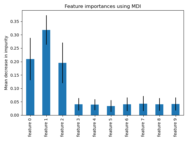
5.4 Gini-Based Feature Importance (Mean Decrease Impurity)
The importance of feature \(j\) in tree \(b\) is the total Gini impurity decrease across all nodes \(t\) where feature \(j\) was used to split, weighted by the fraction of samples reaching each node:
The forest-level importance averages over all \(B\) trees and normalises to sum to 1:
6. Step-by-Step Worked Example
Let's build a tiny Random Forest by hand to see every step concretely. We have 8 training samples with two features (Weather, Wind) and one label (Play tennis?).
| ID | Weather | Wind | Play? |
|---|---|---|---|
| 1 | Sunny | Weak | No |
| 2 | Sunny | Strong | No |
| 3 | Overcast | Weak | Yes |
| 4 | Rain | Weak | Yes |
| 5 | Rain | Weak | Yes |
| 6 | Rain | Strong | No |
| 7 | Overcast | Strong | Yes |
| 8 | Sunny | Weak | No |
Step 1: Bootstrap Sample for Tree 1
Draw 8 samples with replacement. Suppose we get IDs: 1, 3, 3, 4, 5, 6, 7, 8 (ID 3 appears twice; ID 2 is excluded, so it is OOB for Tree 1).
Bootstrap set composition (counting from the original dataset labels): IDs 3, 3, 4, 5, 7 all have Play=Yes (5 samples); IDs 1, 6, 8 have Play=No (3 samples):
| IDs in bootstrap | Play=Yes | Play=No |
|---|---|---|
| 1,3,3,4,5,6,7,8 | 5 (3,3,4,5,7) | 3 (1,6,8) |
Root node Gini: \(G = 1 - (5/8)^2 - (3/8)^2 = 1 - 25/64 - 9/64 = 30/64 \approx 0.469\)
Step 2: Feature Sampling at the Root Split
We have \(p=2\) features. With \(m = \lfloor\sqrt{2}\rfloor = 1\), we randomly pick 1 feature to consider. Suppose we pick Weather.
Split on Weather:
| Weather | Samples (bootstrap) | Yes | No | Gini |
|---|---|---|---|---|
| Sunny | 1, 8 | 0 | 2 | 0.0 |
| Overcast | 3, 3, 7 | 3 | 0 | 0.0 |
| Rain | 4, 5, 6 | 2 | 1 | \(1-(2/3)^2-(1/3)^2 = 0.444\) |
Weighted Gini after splitting on Weather:
Gini reduction: \(0.469 - 0.167 = 0.302\). Since we only had one feature to check, Weather is the split. Tree 1's root node splits on Weather.
Step 3: Grow Tree 1 Fully
After splitting on Weather, the Sunny branch (2 samples, both No) and Overcast branch (3 samples, all Yes) are already pure. No further splits are needed for those branches. The Rain branch (3 samples: Yes, Yes, No) gets another random feature draw and continues recursively.
Step 4: Repeat for Trees 2 through B
Each tree gets its own bootstrap sample and its own random feature draws at every node. For \(B=3\) trees (a minimal forest), we end up with 3 different trees, each with slightly different structure.
Step 5: Predict a New Sample
New sample: Weather=Rain, Wind=Weak. Each tree votes independently:
| Tree | Prediction |
|---|---|
| Tree 1 | Yes |
| Tree 2 | Yes |
| Tree 3 | No |
Majority vote: Yes (2 vs 1). Final prediction: Play tennis = Yes.
7. Out-of-Bag (OOB) Error
One of the most elegant properties of Random Forest is that it comes with a built-in validation estimate for free, without needing a separate validation set.
Because each tree is trained on a bootstrap sample (roughly 63.2% of the data), the remaining 36.8% are genuine unseen samples for that tree. These are the Out-of-Bag (OOB) samples. For each training sample \(i\), we collect all trees whose bootstrap did not include sample \(i\), and use only those trees to predict \(y_i\):
Aggregate across all training samples to get the OOB error:
Breiman showed that OOB error is an approximately unbiased estimate of the test error, roughly equivalent to leave-one-out cross-validation (the approximation tightens as \(B\) grows), but at a tiny fraction of the cost. In scikit-learn, set oob_score=True to compute it automatically.
8. Feature Importance
Random Forest provides two methods to measure which features matter most.
8.1 Mean Decrease Impurity (MDI): built-in, fast
This is the Gini-based importance from Section 5.4: how much each feature reduces impurity across all splits in all trees. It is available via rf.feature_importances_.
Caveat: MDI is biased toward high-cardinality features (features with many unique values, especially continuous ones) because they offer more candidate split points. Do not trust MDI alone for feature selection.
8.2 Permutation Importance: unbiased, slower
Shuffle the values of feature \(j\) in the validation set (or OOB set), breaking any relationship between that feature and the target. Measure how much the model's accuracy drops:
A large drop means the model relied heavily on feature \(j\). Features the model ignores show near-zero drops. Permutation importance is less biased than MDI and works on any estimator. Use sklearn.inspection.permutation_importance.
9. Hyperparameter Guide
| Parameter | scikit-learn name | Default | Effect | Tuning tip |
|---|---|---|---|---|
| Number of trees | n_estimators |
100 | More trees → lower variance, never overfits. Diminishing returns beyond ~200–500. | Start at 100; increase until OOB error plateaus. Time and memory cost scale linearly. |
| Features per split | max_features |
"sqrt" |
Lower → more decorrelated trees, higher bias per tree. Higher → more correlated trees, lower bias per tree. | Try "sqrt", "log2", and a few integer values. Most impactful for accuracy. |
| Max tree depth | max_depth |
None (full) |
Limiting depth reduces variance and training time. Very shallow trees increase bias. | Use None (full trees) when you have enough data. Set 5–15 for noisy datasets. |
| Min samples to split | min_samples_split |
2 | Higher → simpler trees, less overfitting. | Try 2, 5, 10. Especially useful for noisy tabular data. |
| Min samples in leaf | min_samples_leaf |
1 | Ensures leaf nodes have a minimum population; smooths predictions. | Set 1–5 for classification; higher (5–20) for regression. |
| Bootstrap sampling | bootstrap |
True |
False uses the full dataset for every tree (no OOB error available). |
Keep True unless your dataset is very small. |
| OOB score | oob_score |
False |
Computes the free validation estimate using OOB samples. | Always set to True; it costs nothing extra. |
| Class weights | class_weight |
None |
Adjusts influence of each class during training. | Use "balanced" for imbalanced datasets. |
10. Bias–Variance Tradeoff
Every model's generalisation error decomposes as:
A single deep decision tree has low bias (it can fit any boundary) but high variance (it changes dramatically with the training set). Random Forest fixes the variance problem while preserving the low bias of deep trees:
| Model | Bias | Variance | Notes |
|---|---|---|---|
| Shallow tree (max_depth=2) | High | Low | Underfits |
| Deep tree (full) | Low | High | Overfits |
| Random Forest | Low | Low | Averaging reduces variance |
| Gradient Boosting | Very low | Medium | Sequentially reduces bias too, but more prone to overfit |
Adding more trees to a Random Forest never increases bias and only reduces variance (asymptotically). There is no overfitting problem from adding more trees; the only cost is time and memory.
11. Classification vs Regression
Classification
- Each tree votes for a class label (hard vote) or outputs a probability vector (soft vote).
- Split criterion: Gini impurity or entropy.
- Final prediction: majority label or highest mean class probability.
- scikit-learn:
RandomForestClassifier
Regression
- Each tree outputs a real-valued prediction.
- Split criterion: Mean Squared Error (MSE) reduction or Mean Absolute Error (MAE) reduction.
- Final prediction: mean of all tree predictions.
- scikit-learn:
RandomForestRegressor
The split criterion for regression uses MSE:
The best split minimises the weighted MSE of the two children, identical in structure to the Gini criterion for classification.
12. Pros, Cons, and When to Use It
Advantages
- Strong out-of-the-box performance on tabular data. It often beats logistic regression and single trees without any tuning.
- Handles mixed feature types. Continuous and ordinal features work directly. Categorical features must be numerically encoded first (e.g.
OrdinalEncoderorOneHotEncoder) because scikit-learn's implementation requires numeric inputs. - Robust to outliers and noisy features. Averaging across many trees dilutes the effect of any single bad split.
- Built-in feature importance. MDI scores give a fast, interpretable signal about which features matter most.
- Free validation estimate (OOB). You do not need to set aside a separate validation set.
- No feature scaling required. Tree-based splits are invariant to monotone transformations of features.
- Parallelisable. Each tree is trained independently, so training scales linearly across cores using
n_jobs=-1. - Hard to overfit with more trees. Adding more
n_estimatorsonly reduces variance and never increases it.
Disadvantages
- Black box. Individual trees are interpretable, but a forest of 500 trees is not. Use SHAP values for post-hoc explanations.
- Slow to predict at scale. Each prediction must traverse all \(B\) trees. For latency-critical deployments, consider model distillation.
- Memory intensive. The model stores all \(B\) full trees in memory.
- MDI importance is biased. High-cardinality features are systematically overrated. Use permutation importance or SHAP for reliable feature selection.
- Cannot extrapolate. Like all tree-based methods, Random Forest cannot predict beyond the range it saw during training. If the largest target value in training was \(y_{\max}\), it will never predict above \(y_{\max}\).
- Not ideal for very high-dimensional sparse data. On text or NLP features, gradient boosting or linear models often win.
When to choose Random Forest
| Situation | Recommendation |
|---|---|
| Tabular data, mixed types, quick strong baseline needed | Great choice |
| Dataset has noisy features or outliers | Very robust |
| Need built-in feature importance | Use MDI + permutation importance |
| Maximum accuracy on structured data, tuning budget available | Consider XGBoost / LightGBM instead |
| Image, audio, or text data | Use CNNs / Transformers |
| Very large dataset (>10M rows), latency-critical | Consider LightGBM for speed |
| Interpretability is a hard requirement | Use a shallow tree or logistic regression + SHAP |
13. Python Implementation
13.1 Building a Random Forest from Scratch
This section builds a working Random Forest one piece at a time. Each block is explained before the code so you know what it does and why it is written that way.
Part 1: Represent a tree node
A decision tree is a network of nodes. An internal node holds a feature index and a threshold value: samples where feature <= threshold go left; all others go right. A leaf node holds the final predicted class label and has no children. The is_leaf() method lets the prediction function know when to stop traversing and return an answer.
import numpy as np
from collections import Counter

class Node:
    def __init__(self, feature=None, threshold=None, left=None, right=None, value=None):
        self.feature   = feature     # which column to split on
        self.threshold = threshold   # split at this value
        self.left      = left        # subtree for samples where feature <= threshold
        self.right     = right       # subtree for samples where feature > threshold
        self.value     = value       # class label; only set on leaf nodes

    def is_leaf(self):
        return self.value is not None
Part 2: Measure node purity with Gini impurity
Before we can split, we need a way to measure how mixed the labels are at a given node. Gini impurity does this job. It squares the proportion of each class and subtracts from 1. The result is 0 when all samples share the same label (perfectly pure), and rises toward 0.5 as the mix becomes more even.
For example, a node with 6 positives and 4 negatives gives: 1 - (0.6² + 0.4²) = 0.48.
def gini(y):
    counts = Counter(y)
    n = len(y)
    return 1.0 - sum((count / n) ** 2 for count in counts.values())
Part 3: Find the best split at a node
At each node we want the split that reduces impurity the most. This function samples max_features columns at random (the feature-randomness step that decorrelates trees), then tries every unique value in each selected column as a candidate threshold. For each candidate it calculates the Gini gain: the impurity of the parent node minus the weighted average impurity of the two children. The threshold that gives the highest gain is returned.
def best_split(X, y, max_features):
    n_features = X.shape[1]
    # Pick m features at random (feature randomness step that decorrelates trees)
    feature_indices = np.random.choice(n_features, size=max_features, replace=False)

    best_gain, best_feat, best_thresh = -1, None, None

    for feat in feature_indices:
        for thresh in np.unique(X[:, feat]):
            left_mask  = X[:, feat] <= thresh
            right_mask = ~left_mask
            if left_mask.sum() == 0 or right_mask.sum() == 0:
                continue  # skip a threshold that doesn't actually divide the data
            n, n_l, n_r = len(y), left_mask.sum(), right_mask.sum()
            gain = gini(y) - (n_l / n) * gini(y[left_mask]) - (n_r / n) * gini(y[right_mask])
            if gain > best_gain:
                best_gain, best_feat, best_thresh = gain, feat, thresh

    return best_feat, best_thresh
Part 4: Grow one complete tree
grow_tree calls best_split at each node and recurses into both child branches until a stopping condition is met. A node becomes a leaf in three situations: all its samples share the same label (the node is already pure), the tree has reached its maximum allowed depth, or no valid split could be found. The depth argument is incremented on every recursive call so the tree knows how deep it has gone.
def grow_tree(X, y, max_features, max_depth, depth=0):
    # Become a leaf if the data is pure, we hit max depth, or no split exists
    if len(set(y)) == 1 or depth == max_depth:
        return Node(value=Counter(y).most_common(1)[0][0])

    feat, thresh = best_split(X, y, max_features)
    if feat is None:
        return Node(value=Counter(y).most_common(1)[0][0])

    mask  = X[:, feat] <= thresh
    left  = grow_tree(X[mask],  y[mask],  max_features, max_depth, depth + 1)
    right = grow_tree(X[~mask], y[~mask], max_features, max_depth, depth + 1)
    return Node(feature=feat, threshold=thresh, left=left, right=right)
Part 5: Predict with one tree
To predict a single sample, start at the root and walk down the tree. At each internal node, check whether the sample's value for the split feature is less than or equal to the threshold. If yes, go left; if no, go right. Keep going until you reach a leaf, then return its stored class label.
def predict_tree(node, x):
    if node.is_leaf():
        return node.value
    if x[node.feature] <= node.threshold:
        return predict_tree(node.left, x)
    return predict_tree(node.right, x)
Part 6: Assemble the forest
fit loops n_estimators times. Each iteration draws a bootstrap sample (n random row indices with replacement), then calls grow_tree on that sample. Because each tree sees a different bootstrap sample and different random feature subsets at each split, the trees end up different from one another. predict runs every tree on the input, collects all the votes into a matrix, and returns the majority class for each row.
class RandomForestScratch:
    def __init__(self, n_estimators=100, max_features="sqrt", max_depth=None):
        self.n_estimators = n_estimators
        self.max_features = max_features
        self.max_depth    = max_depth or 999
        self.trees        = []

    def fit(self, X, y):
        n = len(y)
        m = int(np.sqrt(X.shape[1])) if self.max_features == "sqrt" else self.max_features
        for _ in range(self.n_estimators):
            idx  = np.random.choice(n, n, replace=True)  # bootstrap: sample with replacement
            tree = grow_tree(X[idx], y[idx], m, self.max_depth)
            self.trees.append(tree)

    def predict(self, X):
        # votes[i][b] = prediction of tree b for sample i
        votes = np.array([[predict_tree(t, x) for t in self.trees] for x in X])
        # For each sample, return whichever class received the most votes
        return np.array([Counter(row).most_common(1)[0][0] for row in votes])
Part 7: Test on the Iris dataset
We test on the Iris dataset: 150 flower samples, 4 numeric features (sepal and petal length and width), and 3 species to predict. We hold out 20% as the test set. With 50 trees and max depth 8, this scratch forest typically reaches 95 to 100% accuracy on the held-out samples.
from sklearn.datasets import load_iris
from sklearn.model_selection import train_test_split
from sklearn.metrics import accuracy_score

X, y = load_iris(return_X_y=True)
X_train, X_test, y_train, y_test = train_test_split(X, y, test_size=0.2, random_state=42)

rf = RandomForestScratch(n_estimators=50, max_depth=8)
rf.fit(X_train, y_train)
y_pred = rf.predict(X_test)
print(f"Scratch RF accuracy: {accuracy_score(y_test, y_pred):.3f}")
# Expected output: Scratch RF accuracy: 0.967  (exact value varies with random state)
13.2 Using scikit-learn for Real Projects
For any real project, use scikit-learn's implementation. It is optimised, parallelised, and handles edge cases that the scratch version ignores. The example below uses the Breast Cancer Wisconsin dataset: 569 samples, 30 numeric features, and a binary label (malignant vs benign). Each step is shown separately so you can see what it produces.
Step 1: Load and split the data
We split 80% for training and 20% for testing. The stratify=y argument ensures both classes appear in the same proportion in both splits, which matters when one class is rarer than the other.
from sklearn.ensemble import RandomForestClassifier
from sklearn.datasets import load_breast_cancer
from sklearn.model_selection import train_test_split, cross_val_score
from sklearn.metrics import classification_report, ConfusionMatrixDisplay
from sklearn.inspection import permutation_importance
import matplotlib.pyplot as plt
import numpy as np

data = load_breast_cancer()
X, y = data.data, data.target
feature_names = data.feature_names

X_train, X_test, y_train, y_test = train_test_split(
    X, y, test_size=0.2, random_state=42, stratify=y
)
print(f"Train: {X_train.shape}   Test: {X_test.shape}")
# Output: Train: (455, 30)   Test: (114, 30)
Step 2: Train the forest
We build 200 trees. With 30 features, max_features="sqrt" means each split considers approximately 5 randomly chosen features. Setting oob_score=True computes a free accuracy estimate from the out-of-bag samples during training, so we can check model quality without touching the test set at all. n_jobs=-1 uses every available CPU core.
rf = RandomForestClassifier(
    n_estimators=200,      # build 200 independent trees
    max_features="sqrt",   # at each split, consider sqrt(30) ~ 5 features
    max_depth=None,        # grow each tree until all leaves are pure
    min_samples_leaf=1,
    oob_score=True,        # estimate accuracy from out-of-bag samples for free
    n_jobs=-1,             # use all CPU cores in parallel
    random_state=42
)
rf.fit(X_train, y_train)

print(f"OOB accuracy (no test data used): {rf.oob_score_:.4f}")
print(f"Test accuracy:                    {rf.score(X_test, y_test):.4f}")
# Typical output:
# OOB accuracy (no test data used): 0.9648
# Test accuracy:                    0.9649
Step 3: Read the classification report
The classification report gives per-class detail. Precision answers: of all samples the model predicted as class X, how many actually were X? Recall answers: of all samples that truly belong to class X, how many did the model correctly identify? F1 is the harmonic mean of precision and recall and summarises both in one number.
print(classification_report(y_test, rf.predict(X_test), target_names=data.target_names))
# Example output:
#               precision    recall  f1-score   support
#    malignant       0.95      0.95      0.95        42
#       benign       0.97      0.97      0.97        72
#     accuracy                           0.96       114
Step 4: Cross-validation for a reliable accuracy estimate
A single train/test split can be lucky or unlucky depending on which samples end up where. Five-fold cross-validation trains and evaluates the model five times on different non-overlapping folds and reports the mean and spread. A tight standard deviation (small number after the +/-) means the score is stable across different data splits.
cv_scores = cross_val_score(rf, X, y, cv=5, scoring="accuracy")
print(f"5-fold CV accuracy: {cv_scores.mean():.4f} +/- {cv_scores.std():.4f}")
# Typical output: 5-fold CV accuracy: 0.9665 +/- 0.0097
Step 5: MDI feature importance
rf.feature_importances_ holds the Mean Decrease Impurity score for each of the 30 features. We sort them from highest to lowest and plot the top 10. A high score means that feature was used frequently at high-impact splits across all 200 trees. Note that MDI tends to overrate continuous features with many unique values, so treat this chart as a rough guide rather than a definitive ranking.
mdi_importance = rf.feature_importances_
sorted_idx = np.argsort(mdi_importance)[::-1][:10]

plt.figure(figsize=(10, 5))
plt.bar(range(10), mdi_importance[sorted_idx])
plt.xticks(range(10), feature_names[sorted_idx], rotation=45, ha="right")
plt.title("Top 10 Features by MDI Importance")
plt.tight_layout()
plt.show()
# Top features are typically: worst radius, worst perimeter, worst area
Step 6: Permutation importance (more reliable)
Permutation importance works differently from MDI. It takes the trained model and the test set, then randomly shuffles the values of one feature at a time, breaking any relationship between that feature and the target. It measures how much accuracy drops. A large drop means the model genuinely relied on that feature. A near-zero drop means the model can manage without it. We repeat the shuffle 10 times per feature and display the spread as a boxplot, which gives a sense of how stable each importance score is.
perm_result = permutation_importance(
    rf, X_test, y_test, n_repeats=10, random_state=42, n_jobs=-1
)
perm_idx = np.argsort(perm_result.importances_mean)[::-1][:10]

plt.figure(figsize=(10, 5))
plt.boxplot(perm_result.importances[perm_idx].T, vert=True, patch_artist=True)
plt.xticks(range(1, 11), feature_names[perm_idx], rotation=45, ha="right")
plt.title("Top 10 Features by Permutation Importance")
plt.tight_layout()
plt.show()
Step 7: Confusion matrix
The confusion matrix shows the full breakdown of predictions. Rows represent the true class; columns represent the predicted class. Numbers on the diagonal are correct predictions. Numbers off the diagonal are errors, and their position tells you exactly which class was confused with which. A well-trained model shows high numbers on the diagonal and values close to zero everywhere else.
ConfusionMatrixDisplay.from_estimator(
    rf, X_test, y_test, display_labels=data.target_names
)
plt.title("Random Forest Confusion Matrix")
plt.show()
13.3 Hyperparameter Tuning with GridSearchCV
Once you have a working model, the next step is finding the best combination of hyperparameters. GridSearchCV tries every combination of values you specify and evaluates each with cross-validation. It then tells you which combination performed best.
The grid below has 3 values of n_estimators, 3 of max_features, 3 of max_depth, and 3 of min_samples_leaf. That is 3 × 3 × 3 × 3 = 81 combinations, each evaluated with 5-fold CV, meaning 405 model fits in total. On the breast cancer dataset this runs in a few minutes.
from sklearn.model_selection import GridSearchCV

param_grid = {
    "n_estimators":     [100, 200, 500],      # more trees = more stable but slower
    "max_features":     ["sqrt", "log2", 0.3], # 0.3 means use 30% of features per split
    "max_depth":        [None, 10, 20],        # None = grow until pure
    "min_samples_leaf": [1, 3, 5],             # higher = simpler trees, less overfitting
}

grid_search = GridSearchCV(
    RandomForestClassifier(n_jobs=-1, random_state=42),
    param_grid,
    cv=5,
    scoring="accuracy",
    n_jobs=-1,
    verbose=1  # prints progress so you can see it is running
)
grid_search.fit(X_train, y_train)

print("Best hyperparameters:", grid_search.best_params_)
print("Best CV accuracy:    ", round(grid_search.best_score_, 4))
print("Test accuracy:       ", round(grid_search.best_estimator_.score(X_test, y_test), 4))
# Example output:
# Best hyperparameters: {'max_depth': None, 'max_features': 'sqrt', 'min_samples_leaf': 1, 'n_estimators': 200}
# Best CV accuracy:     0.967
# Test accuracy:        0.9649
For large datasets where 400+ fits would take too long, replace GridSearchCV with RandomizedSearchCV. Instead of trying all combinations, it samples a fixed number at random, giving a good result in a fraction of the time.
14. Key Takeaways
- Wisdom of crowds: Many imperfect, decorrelated trees outperform any single tree because their errors cancel out.
- Two sources of randomness: (1) bootstrap sampling of rows, (2) random feature subsets at each split. Both are needed. Bootstrapping alone (bagging) leaves trees too correlated.
- Variance falls, bias stays. Adding more trees only helps. There is no overfitting risk from increasing
n_estimators. - OOB error is a free, approximately unbiased test estimate. Always enable it with
oob_score=True. - MDI importance is fast but biased. Use permutation importance or SHAP for reliable feature selection.
- No feature scaling needed. Works with missing values (via imputation) and mixed numeric types.
- Cannot extrapolate beyond the training range. This is a known weakness for regression on out-of-distribution inputs.
References
- Breiman, L. (2001). Random Forests. Machine Learning, 45(1), 5–32. The original paper introducing Random Forest.
- Breiman, L. (1996). Bagging Predictors. Machine Learning, 24(2), 123–140. Introduces bootstrap aggregating.
- Hastie, T., Tibshirani, R., & Friedman, J. (2009). The Elements of Statistical Learning (2nd ed.), Ch. 15. Springer. Rigorous mathematical treatment of Random Forests.
- Louppe, G. (2014). Understanding Random Forests: From Theory to Practice. PhD thesis, University of Liège. Definitive analysis of feature importance and variance reduction.
- Strobl, C. et al. (2007). Bias in random forest variable importance measures. BMC Bioinformatics, 8, 25. Documents MDI bias toward high-cardinality features.
- scikit-learn: Random Forests
- Wikipedia: Random Forest