A Beginner’s Guide to Lasso Regression
1. Introduction
In previous posts, we explored Linear Regression, Ridge Regression, and evaluation metrics like RMSE and R². In this post, we’ll dive into Lasso Regression, short for Least Absolute Shrinkage and Selection Operator.
While Ridge Regression (L2 penalty) shrinks coefficients but keeps them nonzero, Lasso Regression (L1 penalty) can shrink some coefficients to exactly zero. This makes Lasso particularly powerful for feature selection, since it automatically drops irrelevant predictors.
2. The Lasso Cost Function
Ordinary Least Squares (OLS) minimizes squared errors:
$$ J(\beta) = \sum_{i=1}^{n} (y_i - \hat{y}_i)^2 $$
Ridge adds an L2 penalty:
$$ J_{ridge}(\beta) = \sum_{i=1}^{n} (y_i - \hat{y}_i)^2 + \lambda \sum_{j=1}^p \beta_j^2 $$
Lasso instead uses an L1 penalty:
$$ J_{lasso}(\beta) = \sum_{i=1}^{n} (y_i - \hat{y}_i)^2 + \lambda \sum_{j=1}^p |\beta_j| $$
3. Why Does Lasso Set Coefficients to Zero?
Geometrically, Ridge uses a circular (L2 ball) constraint, while Lasso uses a diamond-shaped (L1 ball) constraint. The corners of the diamond tend to align with axes, meaning solutions often hit an axis, forcing coefficients to zero.
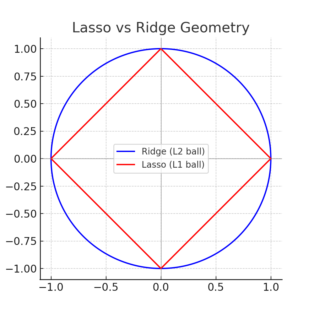
Explanation: Notice how the sharp corners of the diamond (L1) are more likely to “touch” the optimal solution on an axis, forcing coefficients to exactly zero. Ridge’s circle (L2) only shrinks them but rarely sets them to zero.
Soft-thresholding
The Lasso solution is based on a process called soft-thresholding:
$$ S(z, \gamma) = \text{sign}(z) \cdot \max(|z| - \gamma, 0) $$
This pushes small coefficient values to exactly zero. Imagine a V-shaped function: flat at the bottom (coefficients vanish), slanted outside (coefficients shrink).
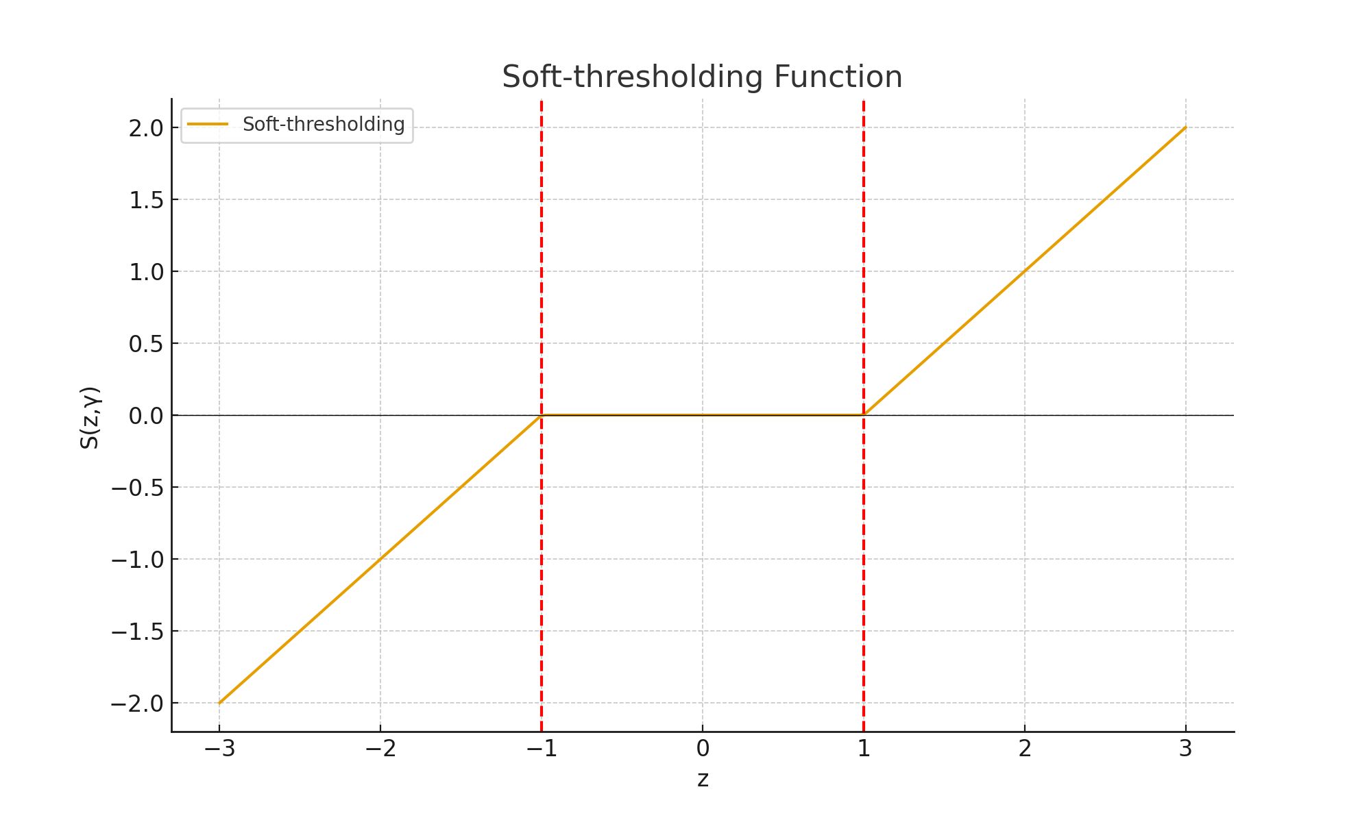
Explanation: Any coefficient smaller than γ in magnitude becomes exactly zero. This is how Lasso performs automatic feature selection.
4. Example with a Tiny Dataset
Let’s use a small dataset so we can follow the math step by step:
| X | y |
|---|---|
| 1 | 2 |
| 2 | 3 |
| 3 | 5 |
| 4 | 7 |
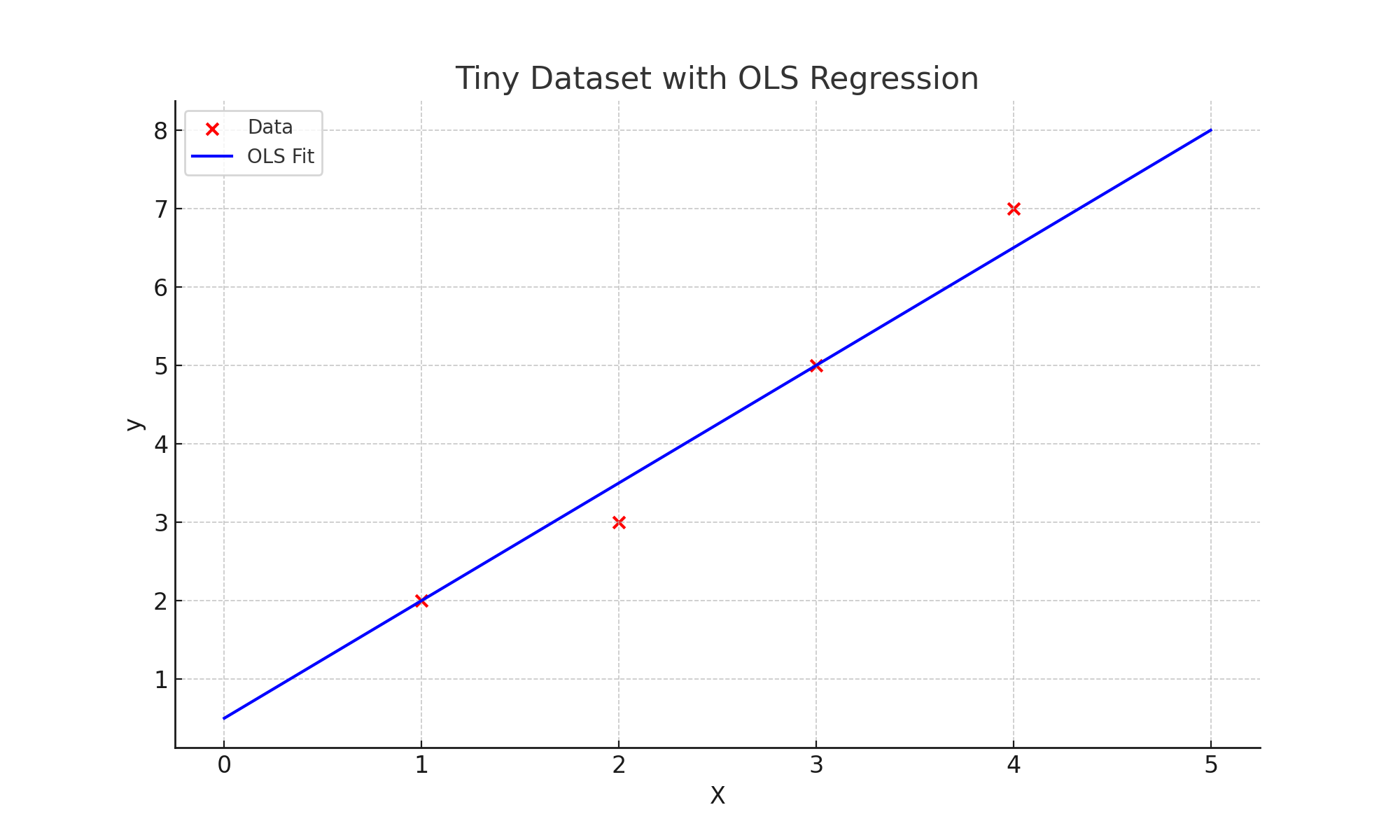
The OLS solution gives approximately:
$$ y = 0.5 + 1.5x $$
Step 1: Compute z
We compute correlation between X and y:
$$ z = \frac{1}{n} \sum x_i y_i = \frac{1}{4}(1*2 + 2*3 + 3*5 + 4*7) = 12.75 $$
Step 2: Apply Penalty
With λ = 1:
$$ \gamma = \frac{\lambda}{2n} = \frac{1}{8} = 0.125 $$
Step 3: Soft-thresholding
$$ \beta_1 = S(12.75, 0.125) = 12.625 $$
The coefficient shrinks slightly. Larger λ shrinks more, eventually reaching zero.
Step 4: Manual Python Demo
import numpy as np

X = np.array([1,2,3,4])
y = np.array([2,3,5,7])
n = len(y)

z = (1/n) * np.sum(X * y)
lam = 1
gamma = lam / (2*n)

def soft_threshold(z, gamma):
    if z > gamma:
        return z - gamma
    elif z < -gamma:
        return z + gamma
    else:
        return 0

beta1 = soft_threshold(z, gamma)
print("z =", z)
print("gamma =", gamma)
print("Updated coefficient β1 =", beta1)
print("Predictions:", beta1 * X)
5. Using Scikit-learn
from sklearn.linear_model import Lasso
import numpy as np
from sklearn.preprocessing import StandardScaler

X = np.array([[1],[2],[3],[4]])
y = np.array([2,3,5,7])

scaler = StandardScaler()
X_scaled = scaler.fit_transform(X)

model = Lasso(alpha=1)
model.fit(X_scaled,y)

print("Intercept:", model.intercept_)
print("Coefficient:", model.coef_)
Explanation: Unlike the manual demo, scikit-learn handles iterative updates and bias term. Notice that coefficients may shrink to zero depending on λ.
6. Visualizations
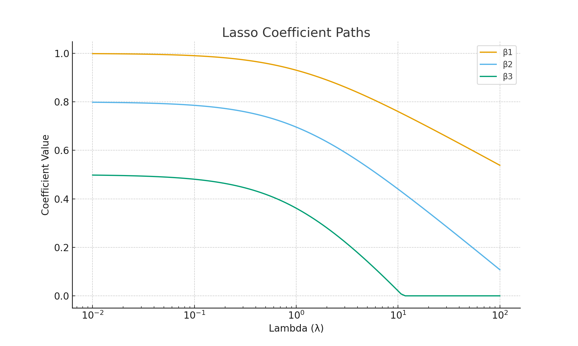
Explanation: Each colored line is a coefficient path. As λ increases (moving right), more coefficients are pulled to zero. This demonstrates Lasso’s ability to perform feature selection.
Explanation: Training error always rises as λ increases (model becomes simpler). Validation error often decreases first (reducing overfitting), then rises again (underfitting). The “U-shape” shows why cross-validation is needed to find the optimal λ.
7. Ridge vs Lasso
| Aspect | Ridge | Lasso |
|---|---|---|
| Penalty | L2 (squared) | L1 (absolute) |
| Effect on Coefficients | Shrinks but never zero | Can shrink to exactly zero |
| Use Case | Handles multicollinearity | Feature selection |
8. Key Takeaways
- Lasso adds an L1 penalty, unlike Ridge which uses L2.
- Lasso can shrink coefficients to zero, performing automatic feature selection.
- Always standardize features before applying Lasso.
- The choice of λ (alpha) is crucial: too small → overfitting, too large → underfitting.
9. Conclusion
Lasso Regression is a powerful extension of linear regression. It combats overfitting through regularization, and simplifies models by removing irrelevant features. Ridge shrinks, Lasso selects.
10. References
- Tibshirani, R. (1996). Regression Shrinkage and Selection via the Lasso.
- Scikit-learn Lasso Docs
- Elements of Statistical Learning (Hastie, Tibshirani, Friedman)