A Beginner’s Guide to Ridge Regression (L2 Regularization)
Linear regression is one of the simplest and most powerful tools in machine learning, but it comes with weaknesses. When predictors are highly correlated (a situation called multicollinearity), or when the dataset is small and noisy, the estimated coefficients can become unstable and extremely large. This instability leads to poor generalization on new data. To overcome this, we use regularization techniques. One of the most popular is Ridge Regression, also known as L2 regularization.
1. Why Do We Need Ridge Regression?
Ordinary Least Squares (OLS) regression estimates coefficients by minimizing the sum of squared errors:
\[ J(\beta) = \sum_{i=1}^{n} (y_i - \hat{y}_i)^2 \]
This works well when predictors are independent and the dataset is large. But when predictors are correlated, \(X^T X\) (the covariance matrix of features) becomes nearly singular. Singular means the matrix cannot be inverted, which makes solving the regression unstable. Small changes in data can then cause large swings in coefficients.
Ridge Regression fixes this by adding a penalty term on the size of the coefficients:
\[ J(\beta) = \sum_{i=1}^{n} (y_i - \hat{y}_i)^2 + \lambda \sum_{j=1}^{p} \beta_j^2 \]
Here, \( \lambda \) is a tuning parameter:
- \(\lambda = 0\): Ridge = OLS (no regularization).
- \(\lambda > 0\): coefficients are shrunk toward zero.
- \(\lambda \to \infty\): all coefficients go toward zero, leading to underfitting.
2. How Do We Derive the Ridge Equation?
The OLS closed-form solution is:
\[ \hat{\beta}_{OLS} = (X^T X)^{-1} X^T y \]
For Ridge, the cost function includes the penalty:
\[ J(\beta) = (y - X\beta)^T (y - X\beta) + \lambda \beta^T \beta \]
Taking the derivative and setting it to zero gives:
\[ (X^T X + \lambda I)\beta = X^T y \]
And solving:
\[ \hat{\beta}_{ridge} = (X^T X + \lambda I)^{-1} X^T y \]
This ensures the matrix is invertible and stabilizes the solution.
3. Manual Example with a Tiny Dataset (Step-by-Step)
Dataset:
| x | y |
|---|---|
| 1 | 2 |
| 2 | 3 |
| 3 | 5 |
| 4 | 7 |
Step 1: Design matrix \(X\) and response \(y\):
\[ X = \begin{bmatrix}1 & 1 \\ 1 & 2 \\ 1 & 3 \\ 1 & 4 \end{bmatrix}, \quad y = \begin{bmatrix}2 \\ 3 \\ 5 \\ 7\end{bmatrix} \]
Step 2: Compute \(X^T X\) and \(X^T y\):
\[ X^T X = \begin{bmatrix}4 & 10 \\ 10 & 30\end{bmatrix}, \quad X^T y = \begin{bmatrix}17 \\ 51\end{bmatrix} \]
Step 3: Add penalty (\(\lambda = 1\)):
\[ X^T X + \lambda I = \begin{bmatrix}5 & 10 \\ 10 & 31\end{bmatrix} \]
Step 4: Inverse:
\[ (X^T X + \lambda I)^{-1} = \frac{1}{55}\begin{bmatrix}31 & -10 \\ -10 & 5\end{bmatrix} \]
Step 5: Multiply (showing the intermediate step):
\[ \begin{bmatrix}31 & -10 \\ -10 & 5\end{bmatrix} \begin{bmatrix}17 \\ 51\end{bmatrix} = \begin{bmatrix}935 - 510 \\ -170 + 255\end{bmatrix} = \begin{bmatrix}425 \\ 85\end{bmatrix} \]
\[ \hat{\beta}_{ridge} = \frac{1}{55}\begin{bmatrix}425 \\ 85\end{bmatrix} = \begin{bmatrix}0.309 \\ 1.545\end{bmatrix} \]
Final model:
\[ \hat{y} = 0.309 + 1.545x \]
4. Manual Calculation in Python (NumPy)
import numpy as np

# Design matrix with intercept
X = np.array([[1,1],[1,2],[1,3],[1,4]])
y = np.array([2,3,5,7])
lmbda = 1

XtX = X.T @ X
Xty = X.T @ y
ridge_matrix = XtX + lmbda * np.eye(XtX.shape[0])
ridge_inv = np.linalg.inv(ridge_matrix)
beta_ridge = ridge_inv @ Xty

print("Ridge coefficients:", beta_ridge)
5. Ridge in Scikit-learn
from sklearn.linear_model import Ridge
import numpy as np

X_feature = np.array([[1],[2],[3],[4]])
y = np.array([2,3,5,7])

ridge = Ridge(alpha=1, fit_intercept=True)
ridge.fit(X_feature, y)

print("Intercept:", ridge.intercept_)
print("Coefficient:", ridge.coef_)
6. Visualizing Ridge Effect
(a) Coefficients vs λ
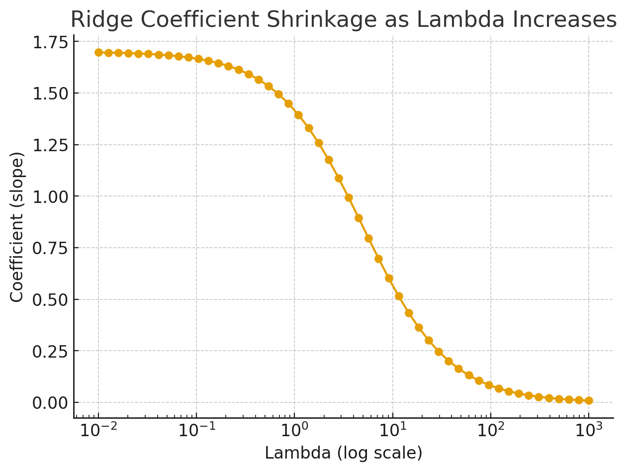
As λ increases, coefficients shrink toward zero. This prevents unstable, extreme values.
(b) Error vs λ
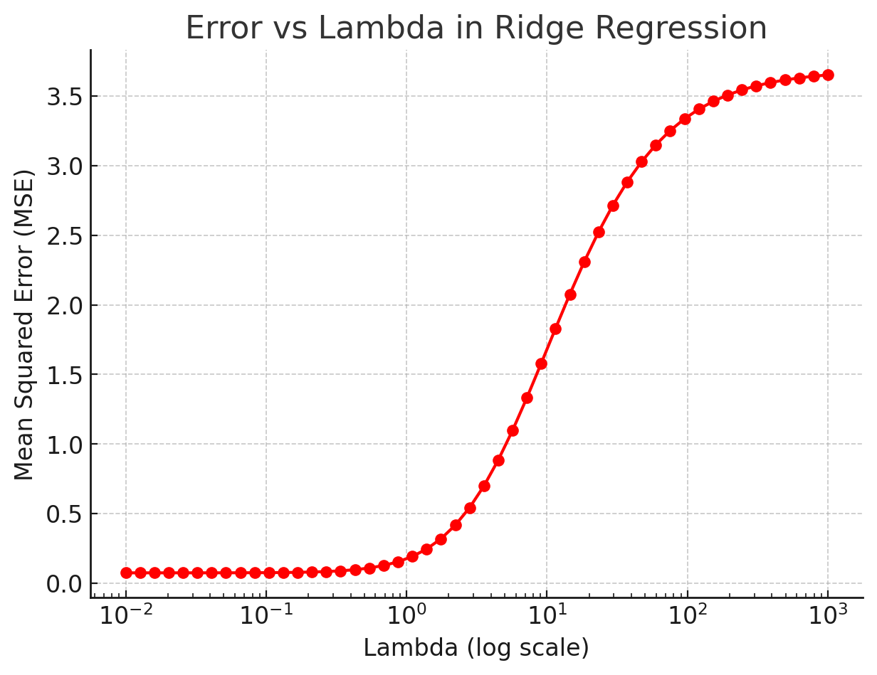
For very small λ, the model can overfit (low bias, high variance). For very large λ, it underfits (high bias, low variance). The sweet spot is at an intermediate λ, which is why we usually pick it using cross-validation.
7. When Should You Use Ridge?
- When features are correlated (multicollinearity).
- When you care more about prediction than coefficient interpretation.
- When you want to reduce variance at the cost of some bias.
8. Pros and Cons
Pros
- Stabilizes regression with correlated predictors.
- Improves prediction accuracy on unseen data.
- Always solvable (matrix invertibility guaranteed).
Cons
- Does not perform feature selection (coefficients never become exactly zero).
- Choice of λ is critical and must be tuned (cross-validation).
- Coefficients are harder to interpret after shrinkage.
9. Key Takeaways
- Ridge adds an L2 penalty that shrinks coefficients.
- It’s useful for noisy, correlated datasets.
- λ controls the bias-variance tradeoff.
- Great entry point for learning regularization.
10. Conclusion
Ridge Regression shows that a slightly biased model can generalize better than an unbiased but unstable model. By controlling coefficient size, Ridge helps create robust and reliable predictive models.
References
- Wikipedia: Ridge Regression
- Scikit-learn Documentation
- Hastie, Tibshirani, Friedman – Elements of Statistical Learning