A Beginner’s Guide to Elastic Net Regression (L1 + L2 Regularization)

1. Quick Intro

Elastic Net combines Ridge (L2) and Lasso (L1) penalties. It’s useful when predictors are correlated — the L2 part stabilizes coefficients while the L1 part encourages sparsity (some coefficients shrink exactly to zero).

\[ \text{Penalty} = \alpha\left[(1-\rho)\tfrac{1}{2}\|\beta\|_2^2 + \rho\|\beta\|_1\right] \]

Here, \(\alpha\) controls the overall strength of regularization, while \(\rho\in[0,1]\) (scikit-learn’s l1_ratio) balances between Ridge (\(\rho=0\)) and Lasso (\(\rho=1\)).

2. Objective Function

The Elastic Net objective minimizes the squared-error loss plus a combination of L1 and L2 penalties:

\[ J_{EN}(\beta) = \sum_{i=1}^n (y_i - \hat y_i)^2 + \alpha\left[(1-\rho)\tfrac{1}{2}\sum_{j=1}^p \beta_j^2 + \rho\sum_{j=1}^p |\beta_j|\right] \]

This approach captures both shrinkage (L2) and variable selection (L1) effects, achieving a balance between interpretability and model stability.

3. Geometric Intuition

Geometrically, Ridge’s penalty region is circular, Lasso’s is diamond-shaped, and Elastic Net lies between them — forming a “rounded diamond.” This shape allows groups of correlated predictors to enter the model together rather than picking just one arbitrarily.

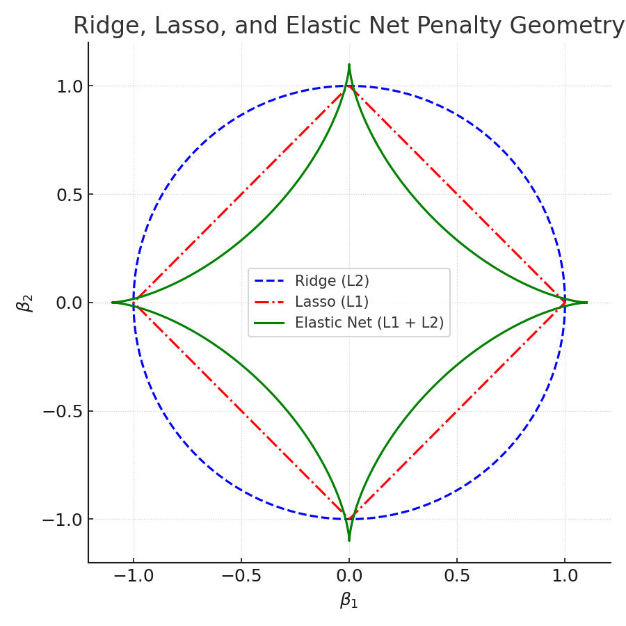
Figure: Ridge (circle), Lasso (diamond), Elastic Net (rounded diamond). The rounded corners encourage grouped feature inclusion.

4. Coordinate Descent & Proximal Step (Concept)

Elastic Net is typically optimized using coordinate descent, which updates one coefficient at a time using a soft-thresholded formula:

\[ \beta_j \leftarrow \frac{1}{1+\alpha(1-\rho)} \; S\!\left( \frac{1}{n}\sum_{i=1}^n x_{ij}(y_i - \hat y_{-j}),\; \frac{\alpha\rho}{n} \right) \]

The L2 term in the denominator stabilizes updates (reducing variance), while the L1 term in the threshold encourages sparsity.

5. Manual Example (Single Feature)

We’ll start with a small dataset to make the math transparent:

X	y
1	2
2	3
3	5
4	7

Assume standardized features, no intercept. Set \(\alpha=1.0\), \(\rho=0.5\), and \(n=4\).

Step-by-Step Calculation

Step 0 — Compute partial correlation \(z\)

\(z = \frac{1}{4}(1\cdot2 + 2\cdot3 + 3\cdot5 + 4\cdot7) = 12.75.\)

Step 1 — Compute L1 threshold \(\gamma\)

\(\gamma = \frac{\alpha\rho}{n} = 0.125.\)

Step 2 — Compute L2 denominator

\(d = 1+\alpha(1-\rho)=1.5.\)

Step 3 — Apply soft-thresholding and divide

\(\beta = \frac{S(z,\gamma)}{d} = \frac{12.625}{1.5} = 8.4167.\)

Step 4 — Compute predictions

\(\hat y = \beta x = [8.42,16.83,25.25,33.67].\)

Note: In practice, features are standardized and an intercept is fitted to prevent inflated coefficients.

6. Manual Python Demo

import numpy as np

X = np.array([1,2,3,4], dtype=float)
y = np.array([2,3,5,7], dtype=float)
n = len(y)

alpha = 1.0
rho = 0.5

z = (1.0/n) * np.sum(X * y)
gamma = alpha * rho / n
denom = 1.0 + alpha * (1.0 - rho)

def soft_threshold(z, gamma):
    if z > gamma: return z - gamma
    elif z < -gamma: return z + gamma
    else: return 0.0

beta = soft_threshold(z, gamma) / denom

print("z =", z)
print("gamma =", gamma)
print("denom =", denom)
print("Updated beta =", beta)
print("Predictions:", beta * X)

7. Scikit-learn Example

from sklearn.linear_model import ElasticNet
from sklearn.preprocessing import StandardScaler
from sklearn.metrics import mean_squared_error, r2_score
import numpy as np

X = np.array([[1],[2],[3],[4]], dtype=float)
y = np.array([2,3,5,7], dtype=float)

scaler = StandardScaler()
Xs = scaler.fit_transform(X)

model = ElasticNet(alpha=1.0, l1_ratio=0.5, fit_intercept=True, max_iter=10000)
model.fit(Xs, y)

y_pred = model.predict(Xs)
print("Intercept:", model.intercept_)
print("Coefficient:", model.coef_)
print("RMSE:", np.sqrt(mean_squared_error(y, y_pred)))
print("R^2:", r2_score(y, y_pred))

8. Visualization Gallery (Five Unique Charts)

1. Actual vs Predicted
   

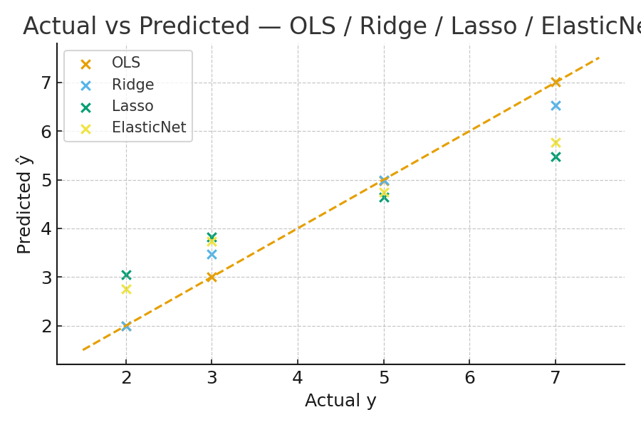
   Compares predicted vs actual target values — helps assess fit quality and bias.

2. Coefficient Path (Regularization Path)
   

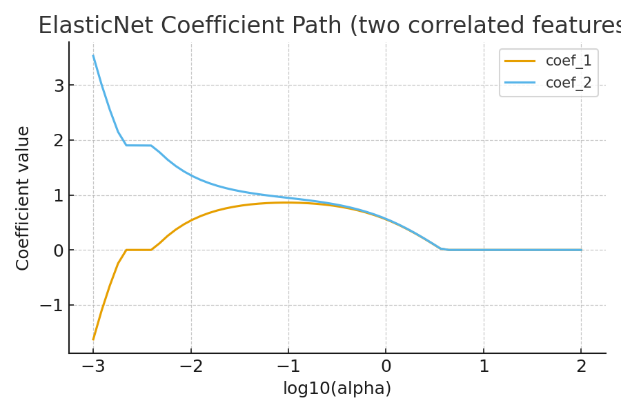
   Shows how each coefficient changes as α increases. Elastic Net’s path is smoother than Lasso’s for correlated predictors.

3. Ridge vs Lasso vs Elastic Net — Coefficients
   

   Highlights shrinkage (Ridge), sparsity (Lasso), and balance (Elastic Net).

4. Residual Plot (Elastic Net)
   

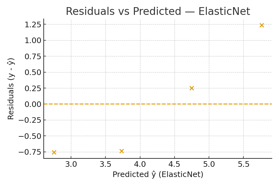
   Visual check for patterns in residuals — non-random patterns indicate model misspecification.

5. Elastic Net Loss Surface
   

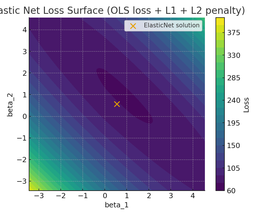
   Conceptual contour showing how Elastic Net blends L1 + L2 regularization with the OLS loss surface.

10. Practical Tips

• Always standardize features before applying regularization.
• Use ElasticNetCV or GridSearchCV to tune alpha and l1_ratio.
• If predictors are highly correlated, Elastic Net groups them instead of arbitrarily choosing one.
• Inspect coefficient paths and validation metrics to confirm model stability.

11. Math Recap

1. \(z = \frac{1}{n}\sum x_i(y_i - \hat y_{-j})\)
2. \(\gamma = \frac{\alpha\rho}{n}\)
3. \(S(z,\gamma) = \operatorname{sign}(z)\max(|z|-\gamma,0)\)
4. \(\beta = \frac{S(z,\gamma)}{1+\alpha(1-\rho)}\)

12. Key Takeaways

• Elastic Net = L1 + L2 blend → balances sparsity and stability.
• Tune alpha and l1_ratio using cross-validation.
• Provides more stable feature selection when predictors are correlated.

---

Related Articles