K-Nearest Neighbors (KNN) — Part 1: Classification

1) What is KNN?

K-Nearest Neighbors (KNN) is a simple, intuitive algorithm that classifies data points by looking at the labels of the closest points in the training set. It's instance-based: nothing is “learned” as coefficients — the algorithm simply stores the examples and uses them at prediction time.

2) Where the equations come from — geometry + voting

KNN uses two simple ideas: distance to measure how close points are, and voting to combine labels from neighbors into a single prediction. Both come from elementary geometry and counting.

Distance: Euclidean (Pythagoras)

In two dimensions the straight-line distance between points \(\mathbf{x}=(x_1,x_2)\) and \(\mathbf{y}=(y_1,y_2)\) follows from the Pythagorean theorem:

Generalising to \(n\) dimensions gives the Euclidean (\(L_2\)) distance:

Intuitively: square differences along each axis, add them (this gives squared straight-line distance), then take the square root to return to the original scale.

Voting: Turning neighbors into a label

Once we have distances, pick the \(k\) nearest neighbors of the query point \(q\) (call this set \(N_k(q)\)). The simplest prediction rule is majority vote (uniform weights):

A more flexible rule is distance-weighted voting, where each neighbor contributes a weight \(w_i\):

Here \(\mathbb{1}(\cdot)\) is the indicator function (1 if the neighbor has class \(c\), else 0), and common choices of weight are:

• Inverse distance: \(w_i = \dfrac{1}{d(q,x_i) + \varepsilon}\) (small \(\varepsilon\) avoids dividing by zero).
• Gaussian: \(w_i = \exp\big(-d(q,x_i)^2/(2\sigma^2)\big)\), which smoothly decays with distance.
• Uniform: \(w_i = 1\) (reduces to majority vote).

3)Step-by-Step Calculation

We'll use a tiny 2D dataset (easy arithmetic) so you can follow every step on paper.

ID	x	y	Class
P1	1	1	A
P2	2	1	A
P3	4	3	B
P4	5	4	B
P5	1	3	A

Query point: \(Q=(3,2)\). We'll compute Euclidean distances to each training point.

Detailed arithmetic (show every step)

1. \(d(Q,P1)=\sqrt{(3-1)^2+(2-1)^2}=\sqrt{4+1}=\sqrt{5}\approx 2.236\)
2. \(d(Q,P2)=\sqrt{(3-2)^2+(2-1)^2}=\sqrt{1+1}=\sqrt{2}\approx 1.414\)
3. \(d(Q,P3)=\sqrt{(3-4)^2+(2-3)^2}=\sqrt{1+1}=\sqrt{2}\approx 1.414\)
4. \(d(Q,P4)=\sqrt{(3-5)^2+(2-4)^2}=\sqrt{4+4}=\sqrt{8}\approx 2.828\)
5. \(d(Q,P5)=\sqrt{(3-1)^2+(2-3)^2}=\sqrt{4+1}=\sqrt{5}\approx 2.236\)

Sorted distances (closest first)

Point	Class	Distance
P2	A	\(\sqrt{2}\approx 1.414\)
P3	B	\(\sqrt{2}\approx 1.414\)
P1	A	\(\sqrt{5}\approx 2.236\)
P5	A	\(\sqrt{5}\approx 2.236\)
P4	B	\(\sqrt{8}\approx 2.828\)

4) Choose k and predict (manual voting)

Pick \(k=3\). The three nearest neighbours are P2 (A), P3 (B) and P1 (A). Counting votes gives A:2, B:1, so KNN predicts A for \(Q\).

Tie handling and why odd k helps

If \(k\) had been 2, we'd have P2 (A) and P3 (B) → a tie. Common tie-breakers are:

• Choose the label of the closest neighbor (1-NN rule).
• Use distance-weighted voting so nearer neighbors influence more.
• Use domain knowledge or random tie-break (not ideal).

Weighted voting (numbers again)

Using inverse-distance weights \(w_i=1/(d_i+\varepsilon)\) with \(\varepsilon=10^{-6}\):

• \(w_{P2}=1/\sqrt{2}\approx 0.707\)
• \(w_{P3}=1/\sqrt{2}\approx 0.707\)
• \(w_{P1}=1/\sqrt{5}\approx 0.447\)

Weighted totals: A = 0.707 + 0.447 = 1.154; B = 0.707. Again A wins.

5) Visual illustration

The figure below shows our five training points and the query point Q(3,2). Points from class A are shown in red and class B in blue. The dashed circle marks the boundary that contains the three nearest neighbors (k = 3).

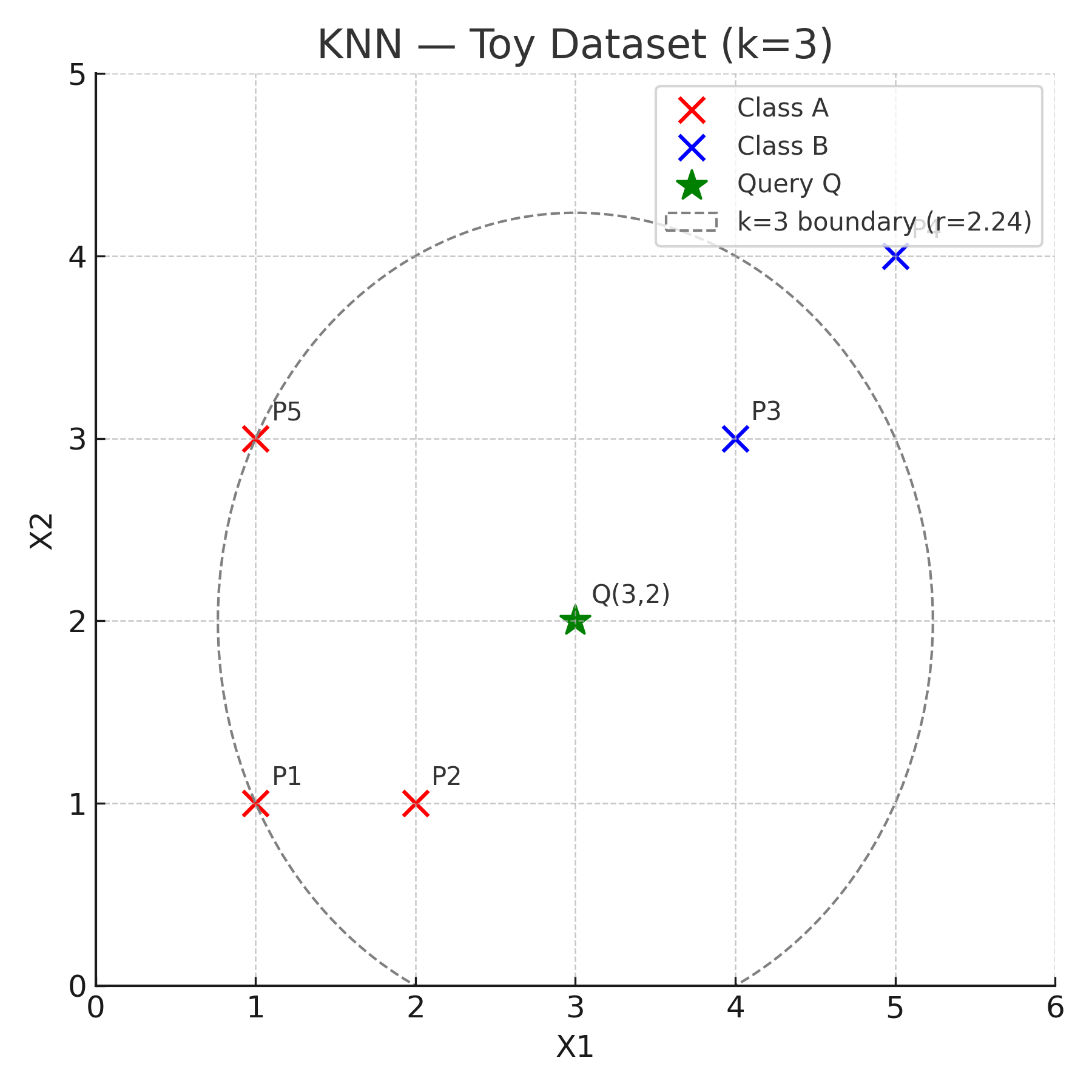
How to read this visual — look for three things:

• Which points are nearest to Q: P2 and P3 are equally close (√2), P1 is next (√5).
• The k=3 circle (dashed): any point inside the circle is among the 3 nearest neighbours of Q.
• Majority vote: two of the 3 neighbours are class A, so the predicted label for Q is A.

6) Practical notes

• Scale your features: KNN uses distances — unscaled features with different units will bias the algorithm.
• Pick k carefully: small k (e.g. 1) → flexible but noisy; large k → smooth but biased. Use cross-validation to choose k.
• Consider weighting: inverse-distance or Gaussian weights often help with noisy training data.
• Distance metric matters: Euclidean is default but L1, Mahalanobis, or cosine may be better in some domains.
• Watch dimensionality: in high dimensions distances concentrate — consider PCA or feature selection first.

7) Complexity & scaling up

Naïve KNN: \(O(n)\) distance computations per query point. For medium/large datasets use spatial indexes: KDTree or BallTree (scikit-learn options) for faster queries in modest dimensions, or approximate nearest neighbour libraries (Annoy, FAISS) for massive/high-dimensional data.

8) Manual Python Calculations

import math
points = {'P1':((1,1),'A'),'P2':((2,1),'A'),'P3':((4,3),'B'),'P4':((5,4),'B'),'P5':((1,3),'A')}
Q = (3,2)

results = []
for name,(coords,label) in points.items():
    dx = Q[0] - coords[0]
    dy = Q[1] - coords[1]
    d = math.sqrt(dx*dx + dy*dy)
    results.append((name, coords, label, d))

results_sorted = sorted(results, key=lambda x: x[3])
print('Sorted neighbours:')
for r in results_sorted:
    print(r)

k = 3
neighbors = results_sorted[:k]
votes = {}
for name,coords,label,d in neighbors:
    votes[label] = votes.get(label,0) + 1
print('\nVotes (majority):', votes)

# weighted votes
w_votes = {}
for name,coords,label,d in neighbors:
    w = 1.0 / (d + 1e-9)
    w_votes[label] = w_votes.get(label, 0) + w
print('Weighted votes:', {k: round(v,3) for k,v in w_votes.items()})

print('\nFinal prediction (majority):', max(votes.items(), key=lambda x: x[1])[0])

9) Optional: Sklearn Library

from sklearn.neighbors import KNeighborsClassifier
import numpy as np
X = np.array([[1,1],[2,1],[4,3],[5,4],[1,3]])
y = np.array(['A','A','B','B','A'])
knn = KNeighborsClassifier(n_neighbors=3)
knn.fit(X,y)
print('Prediction for Q:', knn.predict([[3,2]])[0])

10) Key Takeaways

By doing the arithmetic by hand you can see precisely how KNN decides. The three important knobs are: distance metric, k, and weighting. Change any of them and the decision regions change in predictable ways. For real data, always visualise (when possible), scale features, and use cross-validation to tune \(k\).

References & Further Reading

• Cover, T., & Hart, P. (1967). Nearest neighbor pattern classification.
• Scikit-learn: Nearest Neighbors
• Voronoi diagram (visual intuition)
• StatQuest: KNN Explained Visually

---

Related Articles