Multiple Linear Regression: A Step-by-Step Explanation
In the previous post on Simple Linear Regression, we saw how a single predictor explains a response variable. But in most real problems, one factor is never enough. For house prices, salary prediction, or stock returns, multiple factors interact simultaneously.
This post introduces Multiple Linear Regression (MLR). By the end of this article, you will understand:
- What MLR is and why it matters
- How the regression equation is derived step by step
- A complete worked example with a dataset
- How to interpret the coefficients in plain language
- Key assumptions, pitfalls, and references for deeper study
1. The Idea Behind Multiple Linear Regression
Multiple Linear Regression extends simple regression by allowing more predictors. Instead of drawing a straight line through points on a 2D chart, here we fit a “plane” (or hyperplane in higher dimensions) through multi-dimensional data.
\[ y = \beta_0 + \beta_1 x_1 + \beta_2 x_2 + \cdots + \beta_p x_p + \varepsilon \]
- \(y\): outcome (dependent variable)
- \(x_1, x_2, \dots, x_p\): predictors (independent variables)
- \(\beta_0\): intercept (baseline when predictors are zero)
- \(\beta_j\): slope/partial effect of predictor \(j\)
- \(\varepsilon\): error term (unexplained part)
Interpretation: Each coefficient \(\beta_j\) measures the effect of predictor \(x_j\) on \(y\), while holding all other predictors constant. This “all else being equal” view is what makes MLR powerful. Think of cooking: the final taste depends on many ingredients. To know the effect of salt, you must hold oil and spices fixed — otherwise you confuse the effects.
2. Deriving the Equations
2.1 Least Squares Principle
The main idea is simple: find coefficients so that the predicted values are as close as possible to the actual values. We measure closeness using the sum of squared errors (SSE):
\[ SSE = \sum_{i=1}^n \bigl(y_i - \hat{y}_i\bigr)^2 \]
where the fitted values are:
\[ \hat{y}_i = b_0 + b_1 x_{1i} + b_2 x_{2i} \]
Minimizing SSE means finding the “best compromise line/plane.” To do this, we take partial derivatives with respect to each coefficient, set them to zero, and solve. This produces the normal equations.
\[ \mathbf{b} = (X^\top X)^{-1} X^\top y \]
While the matrix formula looks abstract, it’s just a compact way of solving the system of equations that balance predictor–response relationships. For teaching, we usually compute using deviations from the mean and cross-products — this makes the math more intuitive.
3. Example Dataset
To see this in action, consider a small dataset of house prices with two predictors: area and number of bedrooms. We expect both to increase price, but how much does each matter when we consider them together?
| House | Area (sq.ft) | Bedrooms | Price (k$) |
|---|---|---|---|
| 1 | 1000 | 2 | 250 |
| 2 | 1500 | 3 | 400 |
| 3 | 2000 | 4 | 450 |
| 4 | 2500 | 3 | 500 |
| 5 | 3000 | 5 | 550 |
4. Step-by-Step Solution
Step 1: Compute Means
First, we find averages of each variable — this gives us the “center” of the data:
\[ \bar{x}_1 = 2000, \quad \bar{x}_2 = 3.4, \quad \bar{y} = 430 \]
These means act as reference points. Every other calculation measures how much each observation deviates from these averages.
Step 2: Deviations
Subtract the mean from each observation. Deviations tell us whether each house is above or below average.
\[ x_{1i}' = x_{1i} - \bar{x}_1, \quad x_{2i}' = x_{2i} - \bar{x}_2, \quad y_i' = y_i - \bar{y} \]
Example (House 1):
\[ x_{11}' = -1000, \quad x_{21}' = -1.4, \quad y_1' = -180 \]
This means House 1 is much smaller and cheaper than the average house, with fewer bedrooms too.
| House | x1 | x1 - x̄1 | x2 | x2 - x̄2 | y | y - ȳ |
|---|---|---|---|---|---|---|
| 1 | 1000 | -1000 | 2 | -1.4 | 250 | -180 |
| 2 | 1500 | -500 | 3 | -0.4 | 400 | -30 |
| 3 | 2000 | 0 | 4 | +0.6 | 450 | +20 |
| 4 | 2500 | +500 | 3 | -0.4 | 500 | +70 |
| 5 | 3000 | +1000 | 5 | +1.6 | 550 | +120 |
Step 3: Cross-Products
At this stage, we already have the deviations (how far each value is from its mean). But before jumping to deviations, let’s first see how the raw equations look. They come directly from minimizing the sum of squared errors.
3.1 Least Squares Setup
Regression model:
\[ y_i = b_0 + b_1 x_{1i} + b_2 x_{2i} + e_i \]
We minimize:
\[ SSE = \sum_{i=1}^n (y_i - b_0 - b_1 x_{1i} - b_2 x_{2i})^2 \]
3.2 First-Order Conditions
Setting derivatives equal to zero gives three equations:
\[ \sum (y_i - b_0 - b_1 x_{1i} - b_2 x_{2i}) = 0 \] \[ \sum x_{1i}(y_i - b_0 - b_1 x_{1i} - b_2 x_{2i}) = 0 \] \[ \sum x_{2i}(y_i - b_0 - b_1 x_{1i} - b_2 x_{2i}) = 0 \]
3.3 Expanded Normal Equations
Expanding these yields the normal equations in raw form:
\[ \sum y_i = nb_0 + b_1 \sum x_{1i} + b_2 \sum x_{2i} \] \[ \sum x_{1i}y_i = b_0 \sum x_{1i} + b_1 \sum x_{1i}^2 + b_2 \sum (x_{1i}x_{2i}) \] \[ \sum x_{2i}y_i = b_0 \sum x_{2i} + b_1 \sum (x_{1i}x_{2i}) + b_2 \sum x_{2i}^2 \]
3.4 Switch to Deviation Form
To simplify, we subtract out means. For example:
\[ \sum (x_{1i}y_i) - \frac{\sum x_{1i}\sum y_i}{n} = \sum (x_{1i}'y_i') \]
This conversion removes \(b_0\) from the middle equations and makes everything centered around averages. That’s why we define the following cross-products:
\[ S_{x_1x_1} = \sum (x_{1i}')^2, \quad S_{x_2x_2} = \sum (x_{2i}')^2, \quad S_{x_1y} = \sum (x_{1i}'y_i') \] \[ S_{x_2y} = \sum (x_{2i}'y_i'), \quad S_{x_1x_2} = \sum (x_{1i}'x_{2i}') \]
Each entry is just multiplying deviations row by row. Example (House 1):
\[ (x_1' \text{ for House 1}) \times (y' \text{ for House 1}) = (-1000)(-180) = 180{,}000 \]
Since both values are below average, their product is positive, showing that area and price move together.
| 1 | 1,000,000 | 1.96 | 180,000 | 252 | 1400 |
| 2 | 250,000 | 0.16 | 15,000 | 12 | 200 |
| 3 | 0 | 0.36 | 0 | 12 | 0 |
| 4 | 250,000 | 0.16 | 35,000 | -28 | -200 |
| 5 | 1,000,000 | 2.56 | 120,000 | 192 | 1600 |
| Sum | 2,500,000 | 5.2 | 350,000 | 440 | 3000 |
|---|
Step 4: Normal Equations
Using the corrected cross-product sums, the centered normal equations become:
\[ 2{,}500{,}000 b_1 + 3000 b_2 = 350{,}000 \] \[ 3000 b_1 + 5.2 b_2 = 440 \]
Step 5: Solve
Solving this system step by step, we get:
\[ b_1 \approx 0.125, \quad b_2 \approx 12.5 \]
Interpretation: each sq.ft adds about $125 to price, and each additional bedroom adds about $12,500, holding area constant.
Step 6: Intercept
Finally, we calculate the intercept — the baseline price when predictors are zero (not realistic but mathematically required):
\[ b_0 = 430 - (0.125)(2000) - (12.5)(3.4) \approx 137.5 \]
Final regression equation:
\[ \hat{y} = 137.5 + 0.125 x_1 + 12.5 x_2 \]
Visualizing the Regression Plane
To better understand what this model represents, let’s plot the observed data points (houses) along with the estimated regression plane. Since we have two predictors (area and bedrooms), the fitted model forms a plane in 3D space. Each house sits as a blue dot, and the red plane shows how the regression line balances through the cloud of points.
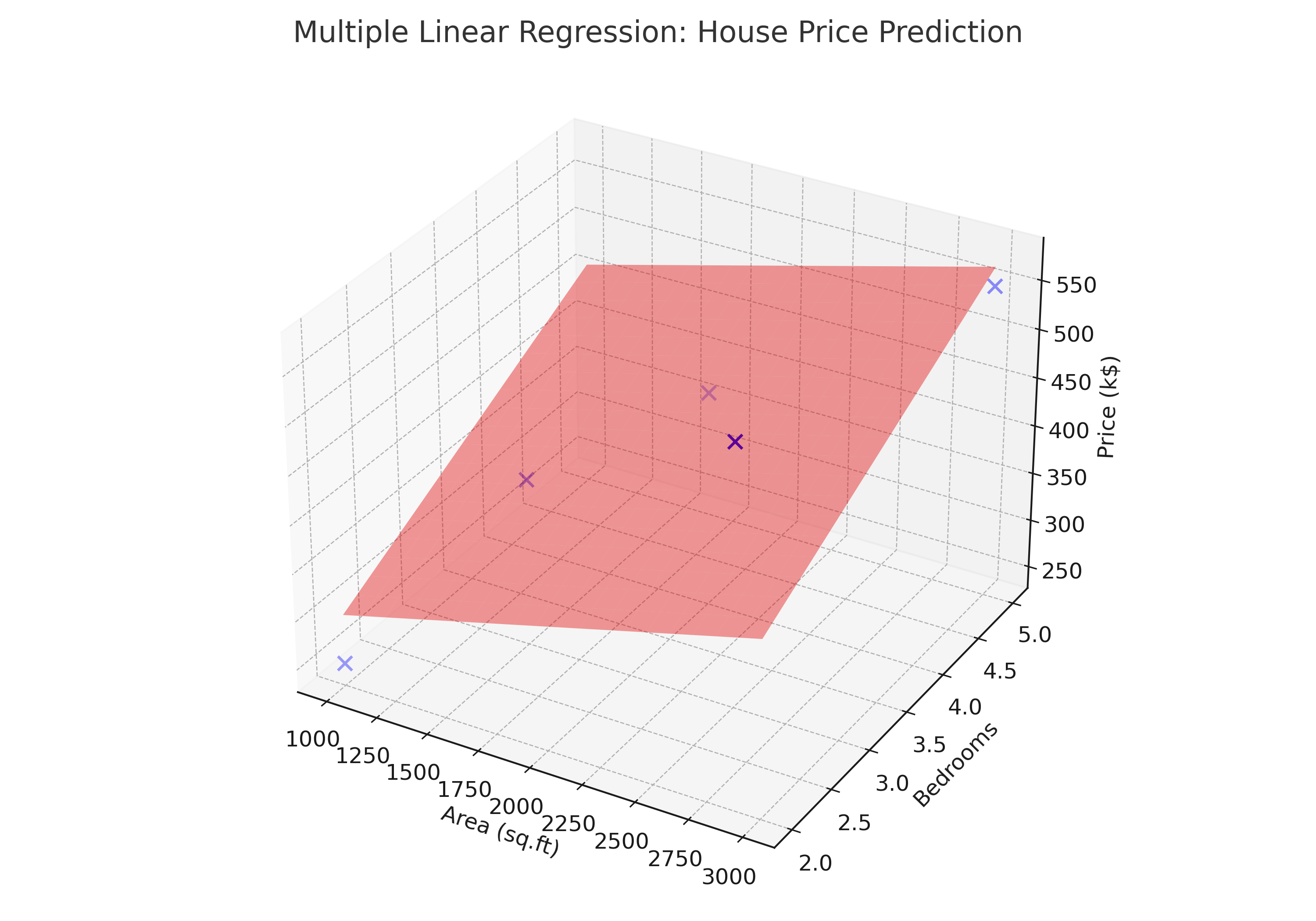
This visualization helps us see the combined effect: as area and bedrooms increase, the regression plane rises, predicting a higher house price. Unlike a simple regression line, the surface shows how multiple predictors work together simultaneously.
5. Prediction Example
Suppose we want to predict the price of a 2200 sq.ft house with 4 bedrooms:
\[ \hat{y} = 137.5 + 0.125(2200) + 12.5(4) = 137.5 + 275 + 50 = 462.5 \ \text{(k\$)} \]
So, our model estimates this house would cost around 463k. This result combines both area and bedroom contributions rather than looking at one factor in isolation.
6. Assumptions & Pitfalls
- Linearity: Predictors are assumed to have straight-line effects on the outcome. If the true relationship is curved, predictions will be off.
- No multicollinearity: Predictors should not be highly correlated. Otherwise, it’s hard to separate their individual effects.
- Homoscedasticity: The spread of errors should be constant. If large houses show more unpredictable prices, this assumption breaks.
- Independence: Each observation (house) should be independent. Prices influenced by neighborhood clustering may violate this.
- Normality (for inference): Residuals should roughly follow a normal distribution if we want valid confidence intervals and hypothesis tests.
Conclusion
Multiple Linear Regression extends the one-predictor case by balancing contributions from multiple variables. We walked through the derivation, solved an example by hand, and saw how to interpret the coefficients.
Despite its simplicity, MLR remains one of the most used tools in statistics and machine learning because it is interpretable, flexible, and applicable across fields — from economics to healthcare.
References
- Montgomery, D.C., Peck, E.A., & Vining, G.G. (2021). Introduction to Linear Regression Analysis (6th ed.). Wiley.
- James, G., Witten, D., Hastie, T., & Tibshirani, R. (2021). An Introduction to Statistical Learning (2nd ed.). Springer (free online).
- Weisberg, S. (2005). Applied Linear Regression (3rd ed.). Wiley.