Simple Linear Regression: A Step-by-Step Explanation

Simple Linear Regression is the simplest but also the most important statistical technique in regression analysis. It helps us describe and predict the relationship between two variables: one independent variable (x) and one dependent variable (y).

The goal is simple: draw a straight line through the data that best represents how y changes when x changes. But to really understand this, we need to carefully walk through the math step by step, not just state the formulas.

In this post, we will:

Derive the regression line from scratch.
Explain what each formula means.
Work through a complete example with housing data.
Clarify why the “n vs n-1” debate doesn’t matter here.

1. The Regression Line

We begin by assuming that the relationship between x and y can be described as:

$$ y = \beta_0 + \beta_1 x $$

Here:

$\beta_0$ (intercept) tells us the expected value of y when x = 0.
$\beta_1$ (slope) tells us how much y changes when x increases by 1 unit.

Our job is to estimate $\beta_0$ and $\beta_1$ from data.

2. The Least Squares Idea

How do we choose the “best” line? The method used is least squares. The idea is:

For each data point, compute the error (residual): $\varepsilon_i = y_i - (\beta_0 + \beta_1 x_i)$
Square these errors so negatives don’t cancel out.
Add them up across all points.

This gives the sum of squared errors (SSE):

$$ SSE = \sum_{i=1}^{n} (y_i - \hat{y}_i)^2 $$

The best line is the one that makes SSE as small as possible.

3. Deriving the Formulas

By taking derivatives of SSE with respect to $\beta_0$ and $\beta_1$ and setting them to zero, we arrive at the normal equations. Solving them gives:

$$ \hat{\beta}_1 = \frac{\sum (x_i - \bar{x})(y_i - \bar{y})}{\sum (x_i - \bar{x})^2}, \quad \hat{\beta}_0 = \bar{y} - \hat{\beta}_1 \bar{x} $$

This means:

The slope is the ratio of how x and y move together (covariance) to how much x varies on its own (variance).
The intercept simply adjusts the line so it passes through the mean point $(\bar{x}, \bar{y})$.

4. Worked Example: Housing Data

Let’s apply this step by step using the following dataset:

Area (x)	Price (y)
1000	250
1500	400
2000	450
2500	500
3000	550

We want to find the regression equation that predicts price (y) from area (x).

Step 1: Compute the Means

$$ \bar{x} = \frac{1000 + 1500 + 2000 + 2500 + 3000}{5} = 2000 $$ $$ \bar{y} = \frac{250 + 400 + 450 + 500 + 550}{5} = 430 $$

The average area is 2000, and the average price is 430. These mean values will act as anchors for our regression line.

Step 2: Compute Deviations from the Mean

Next, we subtract the mean from each value to see how far each point is from the center. These are called deviations, and they form the foundation for covariance and variance.

We already know the means:

\[ \bar{x} = 2000, \quad \bar{y} = 430 \]

Observation	x (Area)	x − 2000	y (Price)	y − 430
1	1000	$-1000$	250	$-180$
2	1500	$-500$	400	$-30$
3	2000	0	450	20
4	2500	500	500	70
5	3000	1000	550	120

So the deviations are:

For $x$: $[-1000, -500, 0, 500, 1000]$
For $y$: $[-180, -30, 20, 70, 120]$

Step 3: Compute Products and Squares

Now we calculate two important things:

The product of deviations $(x_i - \bar{x})(y_i - \bar{y})$ — this tells us how $x$ and $y$ move together.
The square of deviations $(x_i - \bar{x})^2$ — this measures how spread out $x$ is.

Observation	x − 2000	y − 430	(x − 2000)(y − 430)	(x − 2000)²
1	-1000	-180	$(-1000)(-180) = 180{,}000$	$(-1000)^2 = 1{,}000{,}000$
2	-500	-30	$(-500)(-30) = 15{,}000$	$(-500)^2 = 250{,}000$
3	0	20	$(0)(20) = 0$	$(0)^2 = 0$
4	500	70	$(500)(70) = 35{,}000$	$(500)^2 = 250{,}000$
5	1000	120	$(1000)(120) = 120{,}000$	$(1000)^2 = 1{,}000{,}000$
Total			350,000	2,500,000

Thus:

\[ \sum (x_i - \bar{x})(y_i - \bar{y}) = 350{,}000, \quad \sum (x_i - \bar{x})^2 = 2{,}500{,}000 \]

These will now go into the slope formula.

Step 4: Calculate the Slope ($\beta_1$)

The slope formula is:

\[ \beta_1 = \frac{\sum (x_i - \bar{x})(y_i - \bar{y})}{\sum (x_i - \bar{x})^2} \]

We already computed:

$\sum (x_i - \bar{x})(y_i - \bar{y}) = 350{,}000$
$\sum (x_i - \bar{x})^2 = 2{,}500{,}000$

Substitute:

\[ \beta_1 = \frac{350{,}000}{2{,}500{,}000} \]

\[ \beta_1 = 0.14 \]

So, the slope of the regression line is $0.14$. This means: for every additional square foot of house area, the price increases by 0.14 units (in this case, thousands of dollars if we measure prices that way).

Step 5: Calculate the Intercept ($\beta_0$)

The intercept formula is:

\[ \beta_0 = \bar{y} - \beta_1 \bar{x} \]

We know:

$\bar{x} = 2000$
$\bar{y} = 430$
$\beta_1 = 0.14$

Substitute:

\[ \beta_0 = 430 - (0.14 \times 2000) \]

\[ \beta_0 = 430 - 280 \]

\[ \beta_0 = 150 \]

So, the intercept of the regression line is $150$.

Step 6: Conclusion and Interpretation

We now have our final regression equation:

\[ \hat{y} = 150 + 0.14x \]

Let’s carefully interpret what this equation means:

Slope ($\beta_1 = 0.14$): For every increase of 1 unit in area ($x$), the predicted price ($y$) increases by 0.14 units. If the units are square feet for $x$ and thousands of dollars for $y$, then each additional square foot increases the price by \$140.

Intercept ($\beta_0 = 150$): This is the predicted price when $x = 0$. Although a house with 0 area makes no practical sense, the intercept is mathematically required so that the regression line passes through the mean point $(\bar{x}, \bar{y})$. It acts as a baseline adjustment for the equation.

Prediction Example: If we want to estimate the price of a 2500 sq ft house: \[ \hat{y} = 150 + 0.14(2500) = 150 + 350 = 500 \] So the predicted price is 500 (in thousands of dollars, if that’s our unit).

It’s important to remember that regression gives us an average trend. Not every house with 2500 sq ft will cost exactly 500 — but the model predicts that value as the expected price based on the data we used.

5. Visualizing the Regression

Numbers and equations are important, but sometimes it’s easiest to understand regression by looking at a picture. The chart below shows our data points (blue dots) and the fitted regression line (red line).

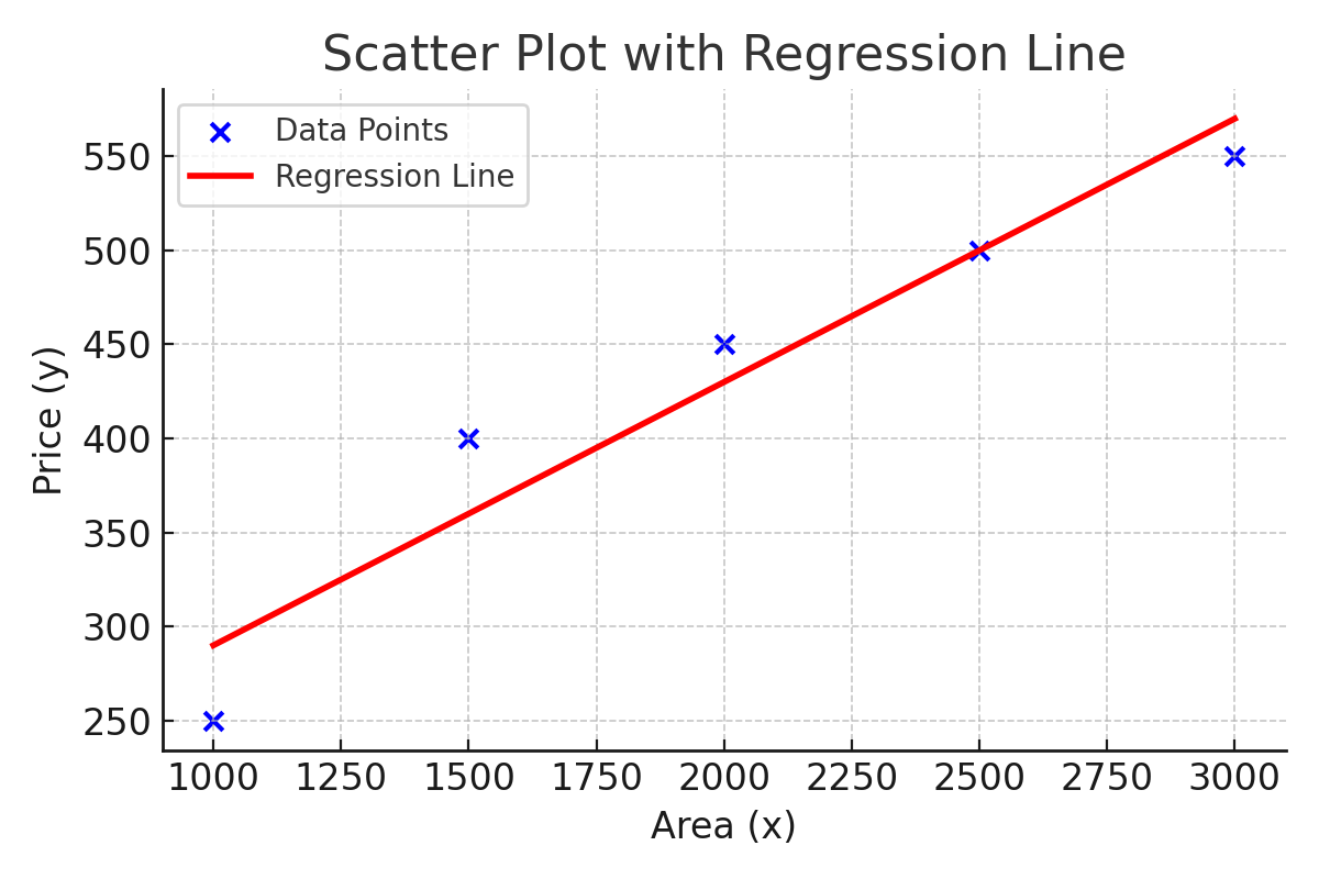
Notice how the line passes through the “middle” of the data points: some points are above, some are below, but overall the line balances them. This is exactly what least squares does — it finds the line that minimizes the total squared vertical distance from all points to the line.

Next, let’s look at the residuals — the differences between the actual prices and the predicted prices. If our regression line is a good fit, the residuals should be scattered around zero without any clear pattern.

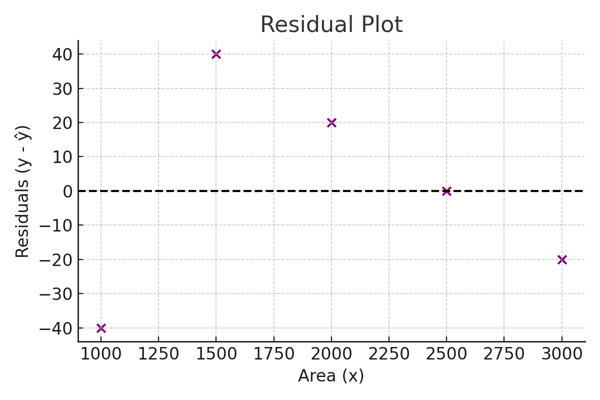
As you can see, the residuals are fairly balanced above and below zero. That means our model does not systematically overpredict or underpredict for small or large houses. This is what we want to see in a simple linear regression.

6. Why Don’t We Use n-1 Here?

In statistics, you may have seen formulas for variance and covariance that divide by n-1 instead of n. This is called Bessel’s correction and is used to make variance an unbiased estimator of the population variance.

But in regression slope:

$$ \hat{\beta}_1 = \frac{\text{Cov}(x,y)}{\text{Var}(x)} $$

Both covariance and variance would use the same denominator (n or n-1), so they cancel out. That’s why it makes no difference here.

However, degrees of freedom do matter later when estimating the error variance:

$$ \hat{\sigma}^2 = \frac{RSS}{n-2} $$

Here, we divide by n-2 because we estimated two parameters ($\beta_0, \beta_1$).

7. Conclusion

We have derived and calculated the regression line step by step. Our final fitted equation was:

$$ \hat{y} = 150 + 0.14x $$

This tells us how house prices grow with area. Going through the math carefully shows how regression is not magic — it’s simply the ratio of covariance to variance, adjusted to pass through the mean point.

And importantly, we clarified that the slope formula doesn’t depend on whether you divide by n or n-1, because the factor cancels.

References

GitHub Repository

Simple Linear Regression Model

Mathematical foundations of ML algorithms.

Simple Linear Regression: A Step-by-Step Explanation

1. The Regression Line

2. The Least Squares Idea

3. Deriving the Formulas

References

- Montgomery, D. C., Peck, E. A., & Vining, G. G. (2021). Introduction to Linear Regression Analysis (6th ed.). Wiley.
- Wooldridge, J. M. (2019). Introductory Econometrics: A Modern Approach (7th ed.). Cengage.
- Freedman, D., Pisani, R., & Purves, R. (2007). Statistics (4th ed.). W. W. Norton & Company.
- Gujarati, D. N., & Porter, D. C. (2009). Basic Econometrics (5th ed.). McGraw-Hill.