RSS Explained: The Complete Beginner’s Guide

Introduction

When building predictive models, we always ask: How close are the predictions to the actual values? One of the earliest and most fundamental error measures in regression is the Residual Sum of Squares (RSS).

RSS plays a central role in least squares regression, diagnostic analysis, and model comparison. While newer metrics like RMSE and MAE are often used for interpretability, RSS is the foundation they build upon.

In this post, we’ll cover:

• What RSS is and why it matters
• Its mathematical definition and intuition
• A worked example
• Visuals that explain RSS step-by-step
• Python code you can use directly
• Strengths and weaknesses of using RSS

---

1. What is RSS?

Residual Sum of Squares (RSS) is the sum of squared differences between observed values and the predictions made by your model:

\( \mathrm{RSS} = \sum_{i=1}^{n} (y_i - \hat{y}_i)^2 \)

• \( y_i \) = actual observed value
• \( \hat{y}_i \) = predicted value from the model
• \( n \) = number of data points

The closer your predictions are to the actual values, the smaller RSS becomes.

Unlike normalized metrics, RSS is scale-dependent: if your dataset doubles, the RSS roughly doubles too.

---

2. Why Squared Residuals?

• Avoid cancellation → Without squaring, positive and negative errors cancel out.
• Penalize big mistakes → Squaring means large errors contribute disproportionately more to RSS.

---

3. Worked Example

X (feature)	Actual y	Predicted ŷ	Residual (y - ŷ)	Squared Residual
1000	250	260	–10	100
1500	400	390	+10	100
2000	450	470	–20	400
2500	500	480	+20	400
3000	550	560	–10	100

\( \mathrm{RSS} = 100 + 100 + 400 + 400 + 100 = 1100 \)

A model with RSS = 0 would mean perfect predictions. Here, our model makes moderate errors, leading to RSS = 1100.

---

4. Visual Intuition

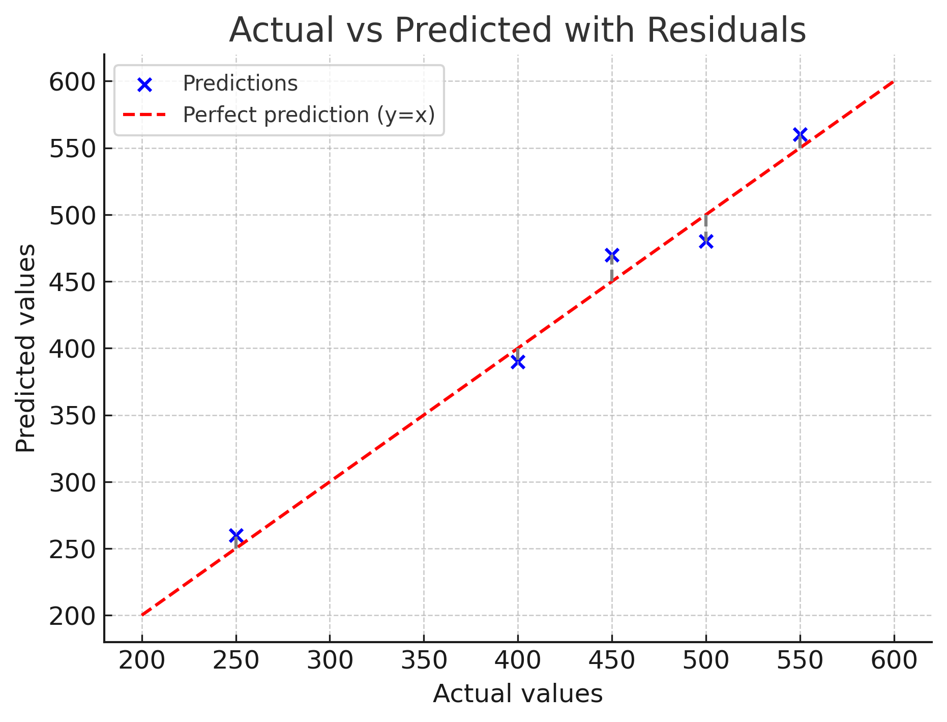
(a) Actual vs Predicted with Residual Lines

In this plot, each blue dot represents a prediction versus its true value. The red dashed line is the "perfect prediction" line (where actual = predicted). The gray dashed vertical lines show the residuals: the gaps between predicted and actual. The RSS is simply the sum of the squares of all these residuals.

---

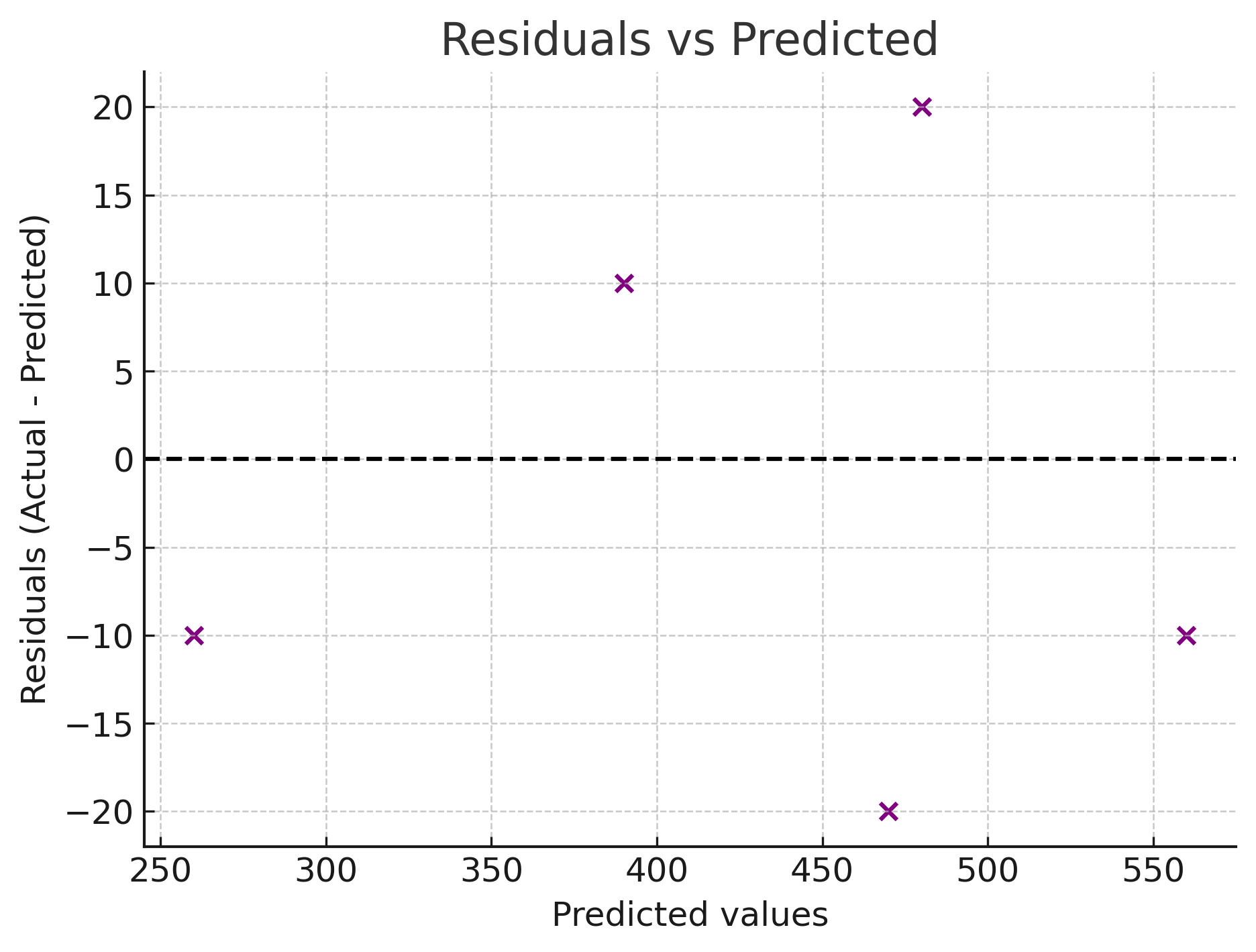
(b) Residuals vs Predicted

Here we plot the residuals (errors) against the predicted values. - The black dashed horizontal line at 0 means "no error." - Points above the line = underestimation (prediction too low). - Points below the line = overestimation (prediction too high).

A good model should show residuals scattered randomly around 0. If you see patterns (like curves, increasing spread, or clustering), it suggests the model has systematic bias. These same residuals are squared and summed to calculate RSS. Large deviations from zero make RSS grow quickly.

---

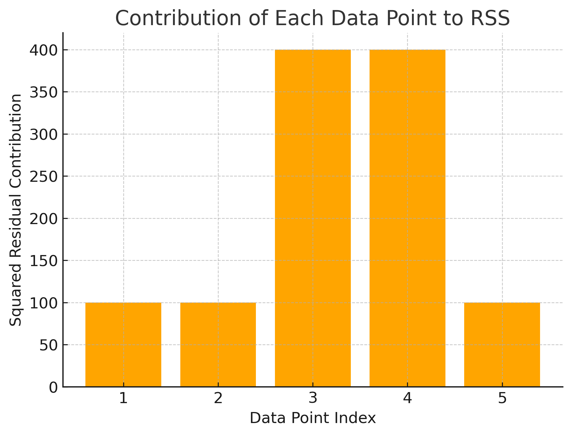
(c) Contribution of Each Data Point to RSS

This bar chart shows how much each observation contributes to the total RSS. - Each bar is the squared residual for a single data point. - Taller bars = larger errors. - Notice how just one or two large errors can dominate the total RSS.

This explains why RSS is sensitive to outliers: a single big mistake can inflate the metric even if most predictions are accurate.

---

5. Python Example

actual = [250, 400, 450, 500, 550]
pred   = [260, 390, 470, 480, 560]

# Compute residuals and RSS
squared_residuals = [(y - y_hat)**2 for y, y_hat in zip(actual, pred)]
RSS = sum(squared_residuals)

# MSE and RMSE
n = len(actual)
MSE = RSS / n
import math
RMSE = math.sqrt(MSE)

print("RSS:", RSS)     # 1100
print("MSE:", MSE)     # 220
print("RMSE:", RMSE)   # ~14.83

This shows how RSS is the building block for other metrics:

• MSE = RSS ÷ number of observations
• RMSE = √MSE (interpretable in the same units as the data)

---

6. Strengths and Weaknesses of RSS

Strengths:

• Forms the basis of least squares regression
• Direct measure of model fit quality
• Useful for comparing nested models

Weaknesses:

• Scale-dependent (grows with dataset size)
• Not interpretable in real-world units
• Sensitive to outliers (a single large error can dominate RSS)

---

7. When to Use RSS

• During model training (objective in OLS regression)
• For diagnostic analysis when adding/removing predictors
• In statistical model comparison

For interpretability in applied ML, RSS is usually paired with RMSE, MAE, or R².

---

Key Takeaways

• RSS = sum of squared residuals.
• Smaller RSS = better fit, but interpretability is limited.
• RSS underpins metrics like MSE, RMSE, and R².
• Always check multiple metrics for a fuller picture of performance.

---

References

• Wikipedia: Residual Sum of Squares
• An Introduction to Statistical Learning (ISLR)
• Regression diagnostics tutorials

---

Related Articles