R² Explained: The Complete Beginner’s Guide

Introduction

When we evaluate regression models, error metrics like RMSE Blogpost tell us how far off predictions are on average. These measures are essential because they quantify the typical size of errors in the same units as the target variable.

But error magnitude alone does not capture the bigger picture. We also want to know how well the model explains the variability in the data compared to a simple baseline (like always predicting the mean). This is where the coefficient of determination, R², comes in. It provides a scale-free measure of goodness of fit, answering the question: “What fraction of the total variation in the outcome does my model explain?”

What is R²?

Informally, R² answers the question: “What fraction of the total wiggle in the data does my model explain?”

R² = 1 — model explains all variability (perfect fit).
R² = 0 — model explains none of the variability (same as predicting the mean).
R² < 0 — model performs worse than the mean predictor (a red flag).

Where R² comes from (variance decomposition)

R² is grounded in a decomposition of variance. Let the actual outcomes be $y_i$, model predictions $\hat{y}_i$, and the sample mean $\bar{y} = \frac{1}{n}\sum_{i=1}^n y_i$.

Define the totals:

Total Sum of Squares (SST) measures total variation in the target around its mean: $$\mathrm{SST} = \sum_{i=1}^n (y_i - \bar{y})^2.$$
Residual Sum of Squares (SSR) (also SSE) measures variation the model fails to explain: $$\mathrm{SSR} = \sum_{i=1}^n (y_i - \hat{y}_i)^2.$$

Then R² is:

$$ R^2 = 1 - \frac{\mathrm{SSR}}{\mathrm{SST}}. $$

Equivalently, R² can be viewed as the fraction of SST captured by the model:

$$ R^2 = \frac{\mathrm{SST} - \mathrm{SSR}}{\mathrm{SST}} = \frac{\mathrm{ESS}}{\mathrm{SST}}, $$

where $\mathrm{ESS}=\mathrm{SST}-\mathrm{SSR}$ is the explained sum of squares.

Detailed example (step-by-step)

We’ll reuse a small toy dataset (house size vs price) to compute R² by hand and explain every step.

Size (sq ft)	Actual price (y)	Predicted price (ŷ)
1,000	250	260
1,500	400	390
2,000	450	470
2,500	500	480
3,000	550	560

Step 1 — compute the sample mean

$$ \bar{y} = \frac{250 + 400 + 450 + 500 + 550}{5} = 430. $$

Step 2 — total sum of squares (SST)

$$ \mathrm{SST} = (250-430)^2 + (400-430)^2 + (450-430)^2 + (500-430)^2 + (550-430)^2 = 53{,}000. $$

This number is the total “wiggle” in the target variable — how far observations deviate from the mean.

Step 3 — residuals and SSR

Residuals: $e_i = y_i - \hat{y}_i$ = [−10, +10, −20, +20, −10]. Squared residuals: [100, 100, 400, 400, 100].

$$ \mathrm{SSR} = 100 + 100 + 400 + 400 + 100 = 1{,}100. $$

Step 4 — compute R²

$$ R^2 = 1 - \frac{1{,}100}{53{,}000} = 0.97925. $$

Interpretation: the model explains about 97.9% of the variance in this toy dataset.

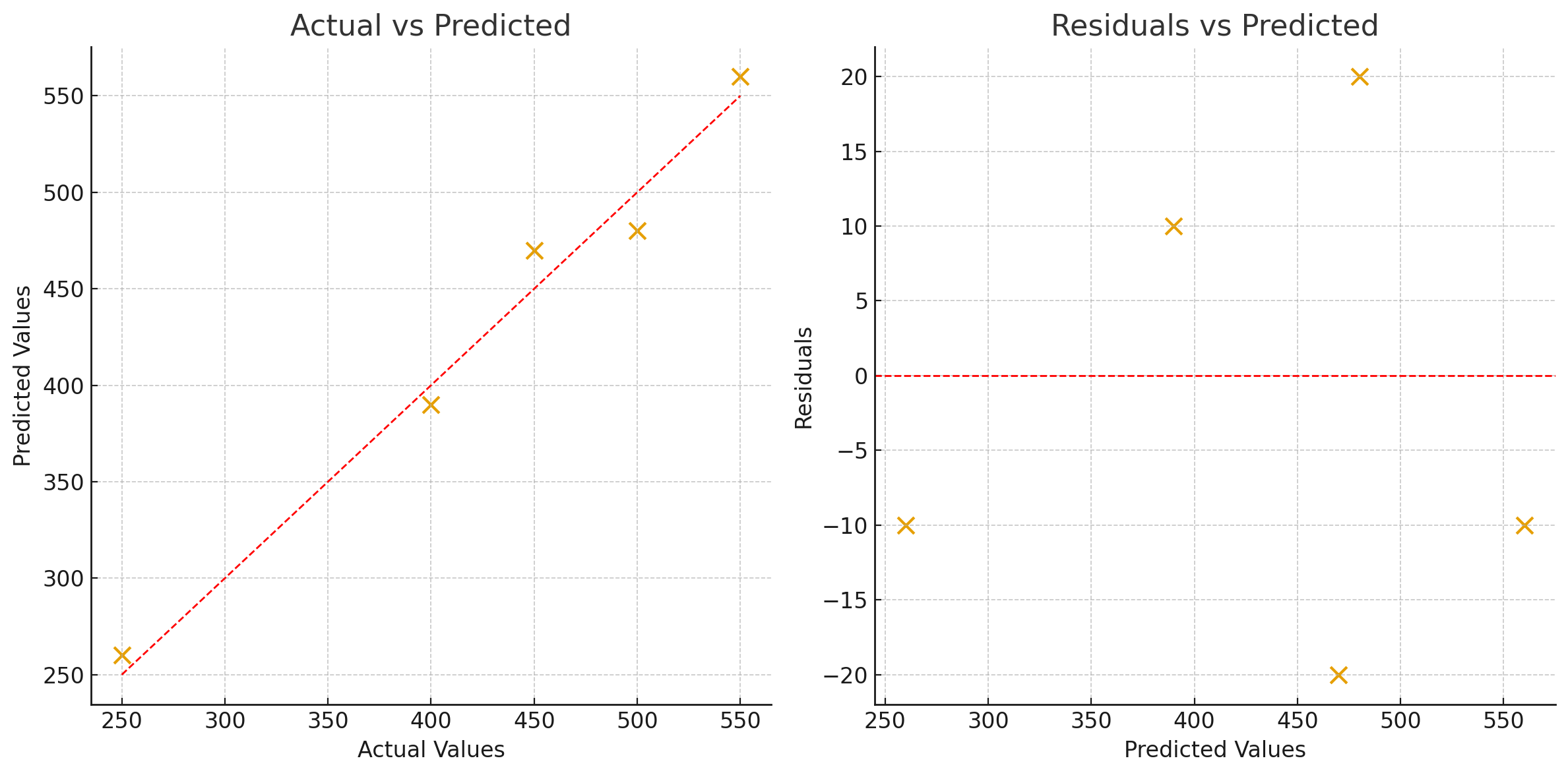
Visual intuition (plots)

Below are three plots that together capture the same information R² summarises. I have generated PNG files and included them in the assets folder.

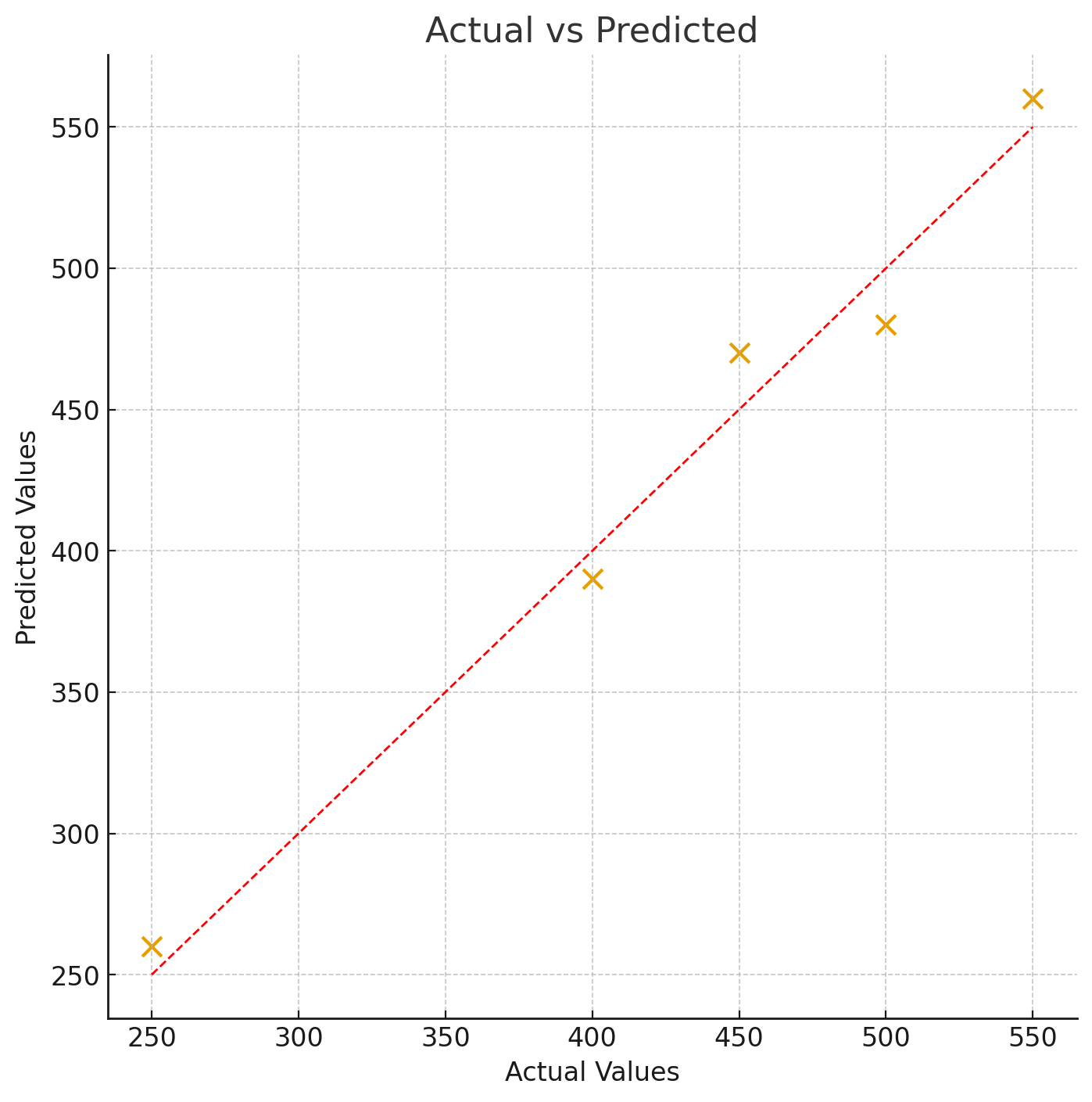
Actual vs Predicted

Predicted values on the vertical axis and actual values on the horizontal axis. The dashed diagonal is the perfect-fit line.

Actual vs Predicted scatter

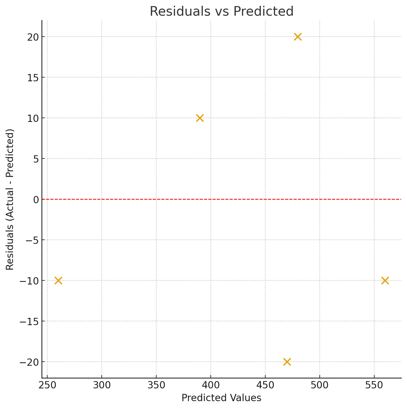
Residuals vs Predicted

Residuals plotted against predicted values. Good models have residuals randomly scattered around zero.

Residuals vs predicted

Combined view

Left: actual vs predicted. Right: residuals vs predicted — a compact diagnostic panel.

Combined visualization

Common questions:

Why can R² be negative?

R² becomes negative when SSR > SST — i.e. the model’s predictions are worse (in squared error sense) than simply predicting the sample mean for every observation. Negative R² is a clear indicator of a poorly specified model or that the model is extrapolating badly for the dataset used.

Adjusted R² — accounting for number of predictors

When you add more predictors to a regression model, R² never decreases even if the new predictor is useless. Adjusted R² corrects for this by penalising model complexity:

$$ R^2_{adj} = 1 - (1 - R^2) \frac{n - 1}{n - p - 1}, $$

where $n$ is the number of samples and $p$ the number of predictors (excluding the intercept). Use adjusted R² to compare models with different numbers of features.

R² vs RMSE (and other error metrics)

R² is unitless and interprets variance explained, whereas RMSE/MAE provide absolute error magnitudes in the same units as the target. A model can have a high R² but still produce large RMSE if the target variance is huge. Always consider both.

When is R² misleading?

Small sample sizes — training variance can make R² unstable.
Heteroskedasticity — variance of errors changes across x, undermining interpretation.
Nonlinear relationships not captured by the model — a linear model may have low R² even when a nonlinear pattern exists.
Time-series forecasts — R² may be less informative without accounting for autocorrelation and fit on holdout sets.

Practical recommendations

Report R² alongside RMSE/MAE and residual diagnostics.
Use adjusted R² when comparing models with different numbers of predictors.
Always validate R² on a held-out test set (or use cross-validation).
For interpretability, convert R² to percentage: e.g. R² = 0.65 → “65% of variance explained”.

Python code sample


        import numpy as np
        from sklearn.metrics import r2_score
        import matplotlib.pyplot as plt

        # Data
        actual = np.array([250, 400, 450, 500, 550])
        pred   = np.array([260, 390, 470, 480, 560])

        # Manual computation
        y_mean = actual.mean()
        sst = np.sum((actual - y_mean)**2)
        ssr = np.sum((actual - pred)**2)
        r2 = 1 - ssr / sst
        print('Manual R²:', r2)

        # sklearn
        print('sklearn R²:', r2_score(actual, pred))

Key takeaways

R² measures proportion of variance explained by the model — intuitive and widely used.
Use adjusted R² to account for number of predictors.
Pair R² with RMSE/MAE and residual plots for a full diagnostic.
Validate on holdout data — don’t trust training R² alone.

References

James, G., Witten, D., Hastie, T., & Tibshirani, R. (2013). An Introduction to Statistical Learning. Springer. [Book link]
Chicco, D., Warrens, M. J., & Jurman, G. (2021). The coefficient of determination R². Biometrics, 77(2), 781–791. [DOI]
Scikit-learn: r2_score

A Beginner’s Guide to R-Squared (R²)

Evaluation Metrics

R² Explained: The Complete Beginner’s Guide

Introduction

What is R²?

Where R² comes from (variance decomposition)

Detailed example (step-by-step)